Data Mining
projects from the course 'Data Mining' at Leiden University
Recommender Systems - MovieLens 1M Dataset
In this assignment, we implemented several recommendation algorithms using the MovieLens 1M dataset, which contains 1,000,209 ratings of approximately 3,900 movies made by 6,040 MovieLens users who joined MovieLens in 2000. The ratings are on a 5-star scale (whole-star ratings only). Each user has at least 20 ratings. The dataset also includes user information about their gender, age, occupation and zip-code, and movie information about the title and genres. The whole dataset can be downloaded from here.
For this assignment, we used the following algorithms:
- Naive Approaches: global average rating, average rating per item, average rating per user, and an “optimal” linear combination of the two averages (per user and per item), with and without the parameter γ.
- UV matrix decomposition algorithm
- Matrix Factorization with Gradient Descent and Regularization
For the validation, we used a 5-fold cross-validation, where the dataset was randomly divided into 5 parts, and each part was used as a test set once while the other parts were used as training sets. The RMSE and MAE were calculated for each fold and averaged over the 5 folds. This is a common technique to evaluate the performance of a model and make sure it generalizes well to unseen data.
During training, we kept track of the execution time and memory usage of each model, as well as the RMSE and MAE on each epoch. The plots below show the RMSE and MAE of the UV decomposition and Matrix Factorization models during training.
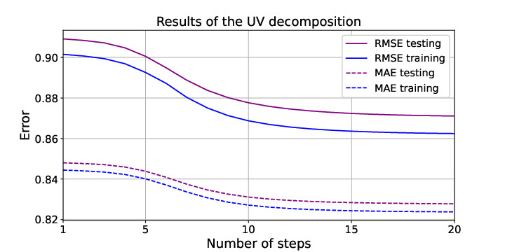
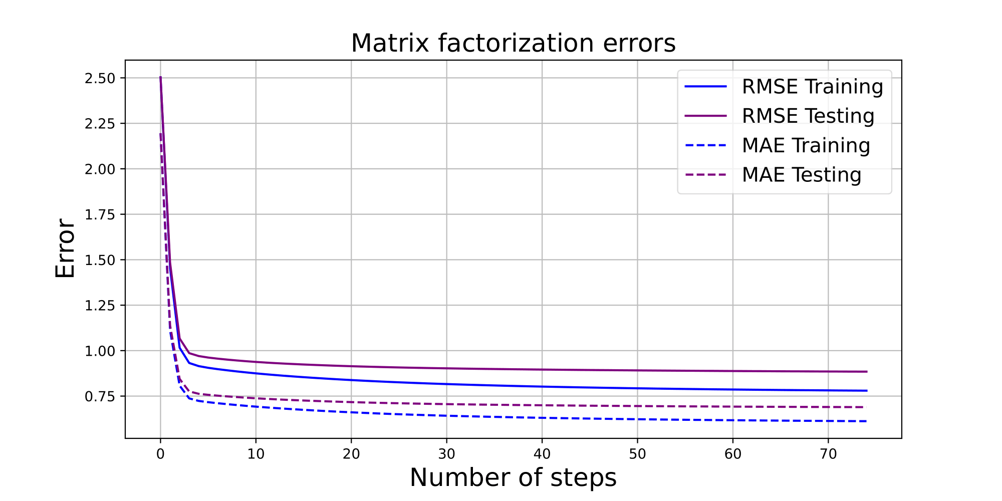
The final comparison of the models shows that the Matrix Factorization model performed the best, with the lowest RMSE and MAE on the test set. The UV Decomposition model was not better than some of the naive approaches, which makes it a poor choice for this dataset. The final performance of the models, with the execution time and memory usage, is shown in the plots below.
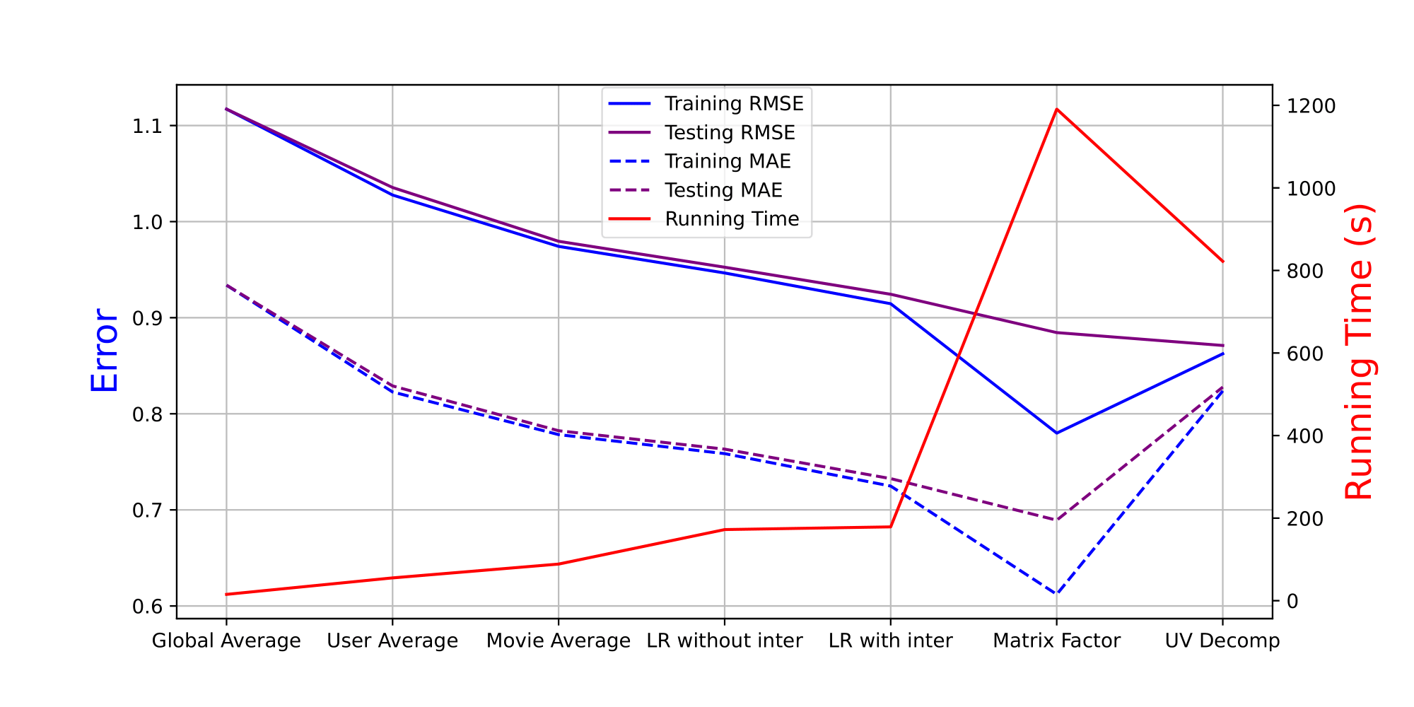
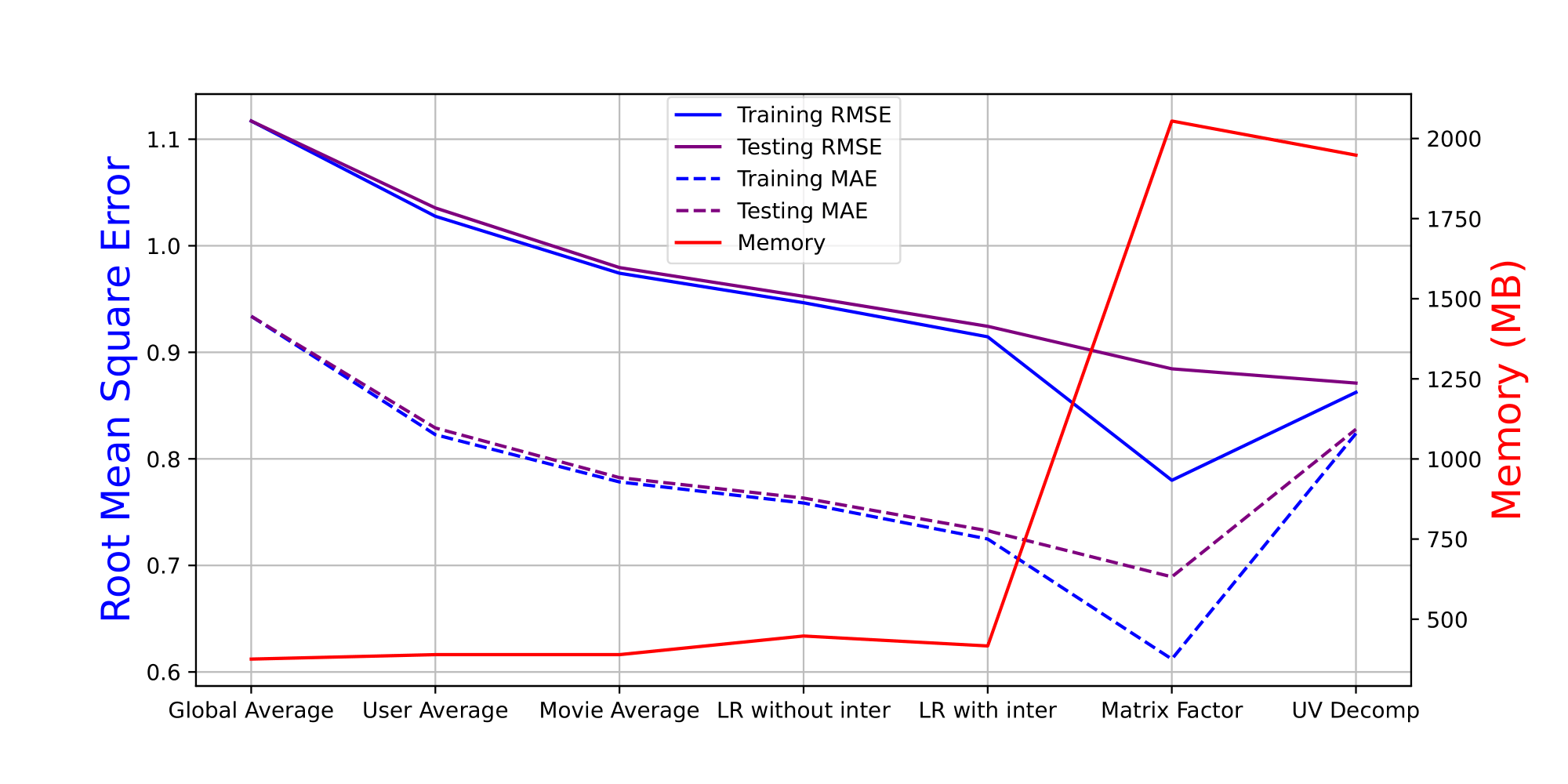
The results can, also, be summarized in a table:
| Model | RMSE Test | MAE Test | Execution Time (s) | Memory (MB) |
|---|---|---|---|---|
| Global Average | 1.117 | 0.934 | 15.330 | 375.5 |
| Movie Average | 0.980 | 0.782 | 88.707 | 389.4 |
| User Average | 1.035 | 0.829 | 55.218 | 389.4 |
| Lin Reg with intercept | 0.924 | 0.733 | 178.778 | 416.6 |
| Lin Reg without intercept | 0.953 | 0.763 | 172.274 | 447.5 |
| UV Decomposition | 0.871 | 0.828 | 822.069 | 1948.0 |
| Matrix factorisation | 0.885 | 0.689 | 1190.862 | 2054.6 |
The next part of the assignment was to use dimensionality reduction techniques to visualize the data. We used three different techniques:
- PCA (Principal Component Analysis)
- t-SNE (t-Distributed Stochastic Neighbor Embedding)
- UMAP (Uniform Manifold Approximation and Projection)
We first used the dimensionality reduction techniques to cluster the users based on their gender and see if the clusters were separable. The plots below show the results of the three techniques, where the colors represent the gender of the users.
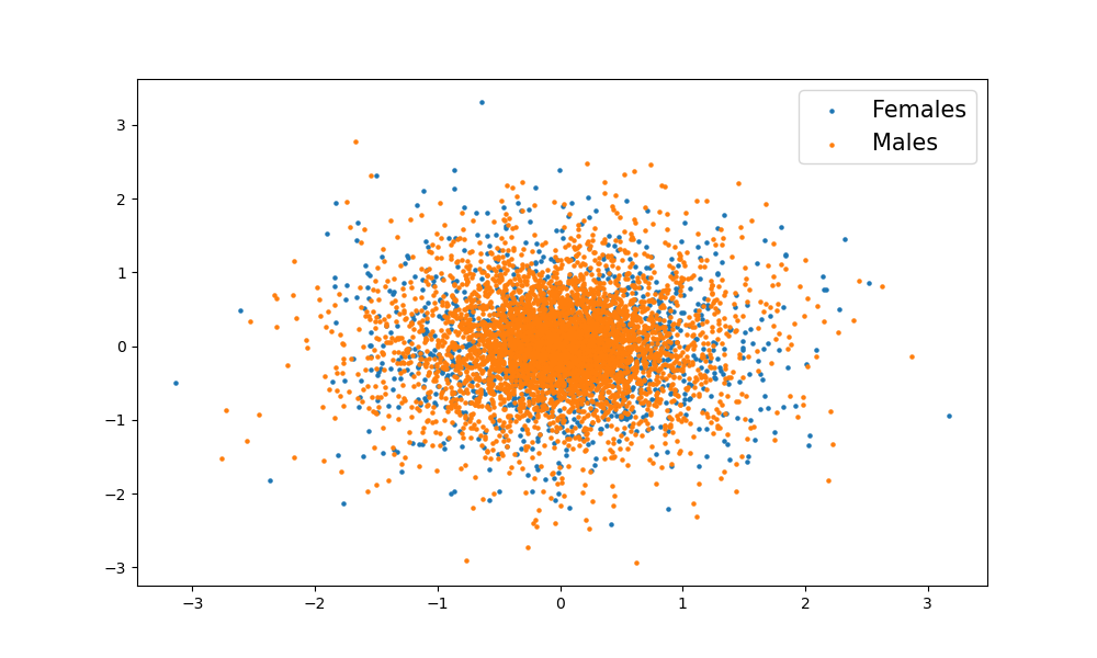
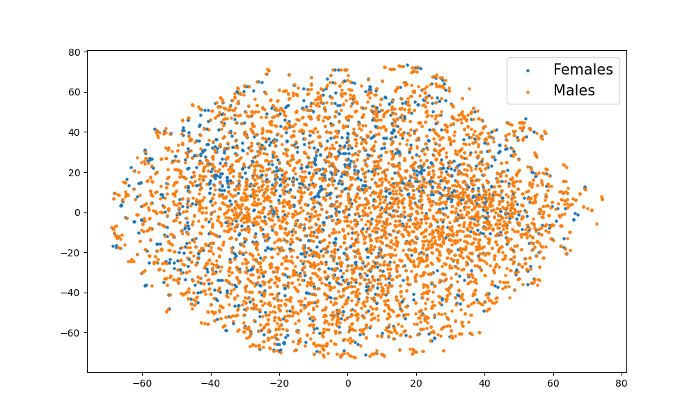
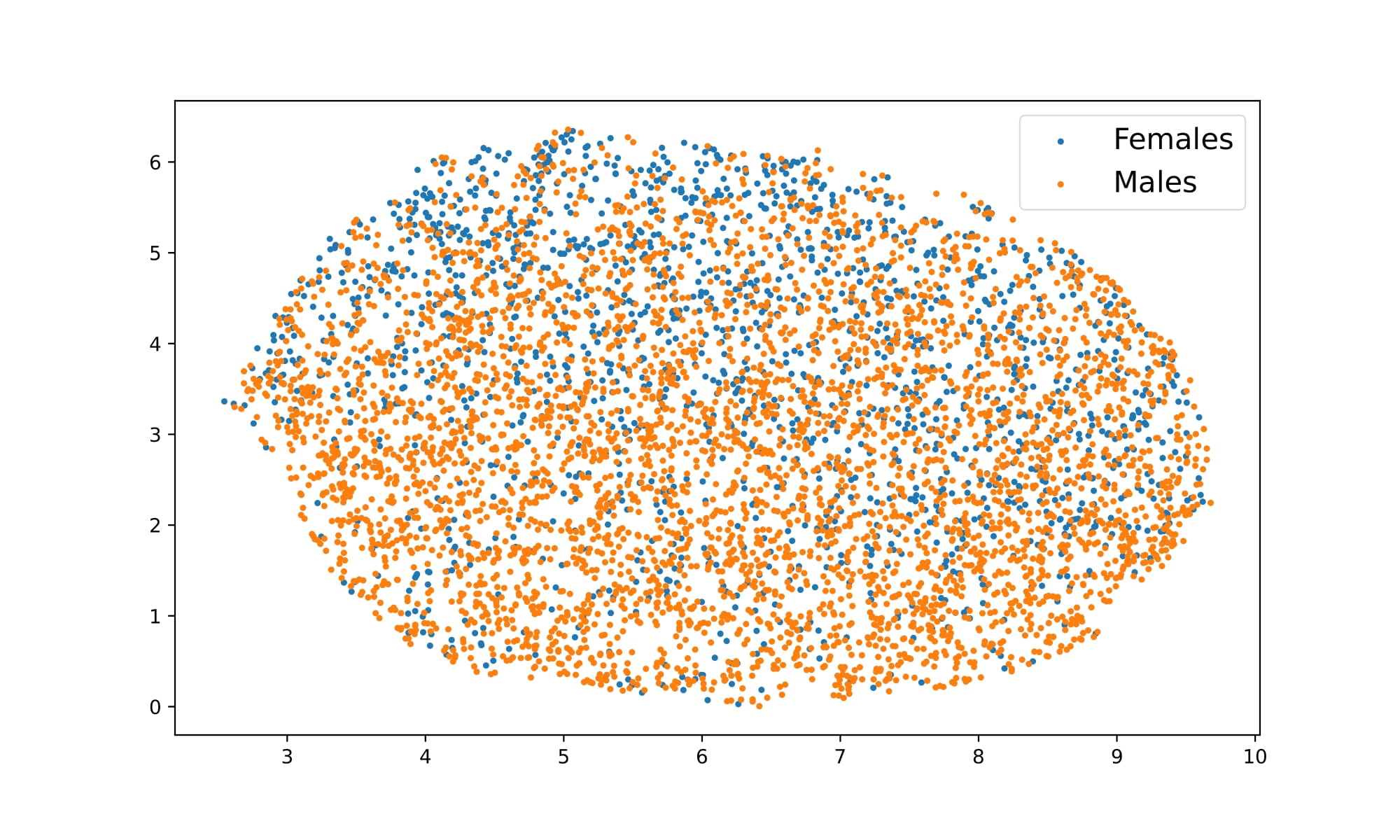
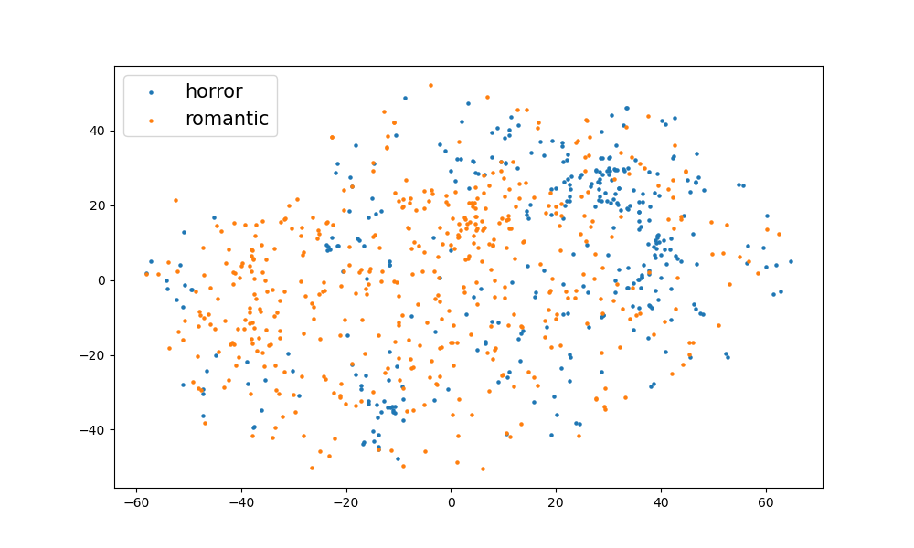
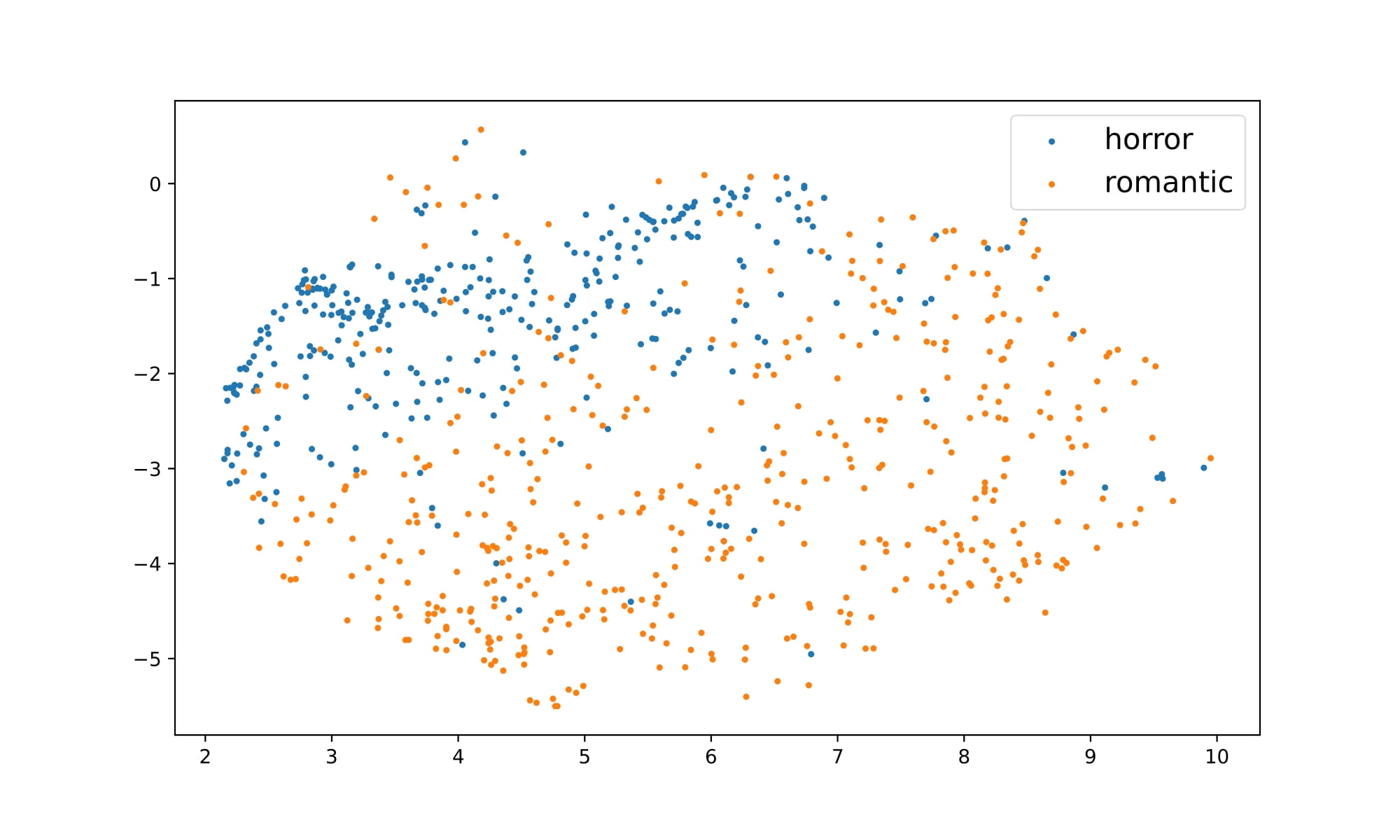
As it is clear, the different genders are not separable using these techniques. We can also see that the PCA plots are not very informative, as all the points are clustered together. We created many more plots using the same techniques and different features. On the plots below, we clustered the movies based on 2 genres (horror and romantic) using t-SNE and UMAP. In this case we can see that the clusters are more separable, especially using UMAP.
In conclusion, this assignment was a great opportunity to learn about recommendation algorithms and dimensionality reduction techniques. We were able to implement several models and compare their performance on the MovieLens 1M dataset. We also learned how to use PCA, t-SNE, and UMAP to visualize the data and see if clusters can emerge from different features of the dataset. The results were very informative and helped us understand the strengths and weaknesses of each model and technique. For more details, you can check the full report here. The full code can be found on my GitHub repository.
Predict Future Sales - Kaggle Competition
In this assignment, we participated in the Kaggle competition “Predict Future Sales”, where we had to predict total sales for every product and store in the next month. The dataset consists of daily sales data, provided by one of the largest Russian software firms - 1C Company. The task was to predict the total sales for every product and store in the next month. The dataset can be downloaded from here.
Each item in the dataset has a unique identifier, which is a tuple of the shop_id and item_id. The dataset also includes:
- item_category_id: unique identifier of item category
- item_cnt_day: number of products sold.
- item_price: current price of an item
- date: date in format dd/mm/yyyy
- date_block_num: a consecutive month number starting from January 2013 (0) to October 2015 (33)
- item_name: name of item
- shop_name: name of shop
- item_category_name: name of item category
The aim of the assignment was to perform exploratory data analysis (EDA) on the dataset, preprocess the data, and implement several existing forecasting models. We used the following models:
- LGB (Light Gradient Boosting)
- XGB (Extreme Gradient Boosting)
- Random Forest
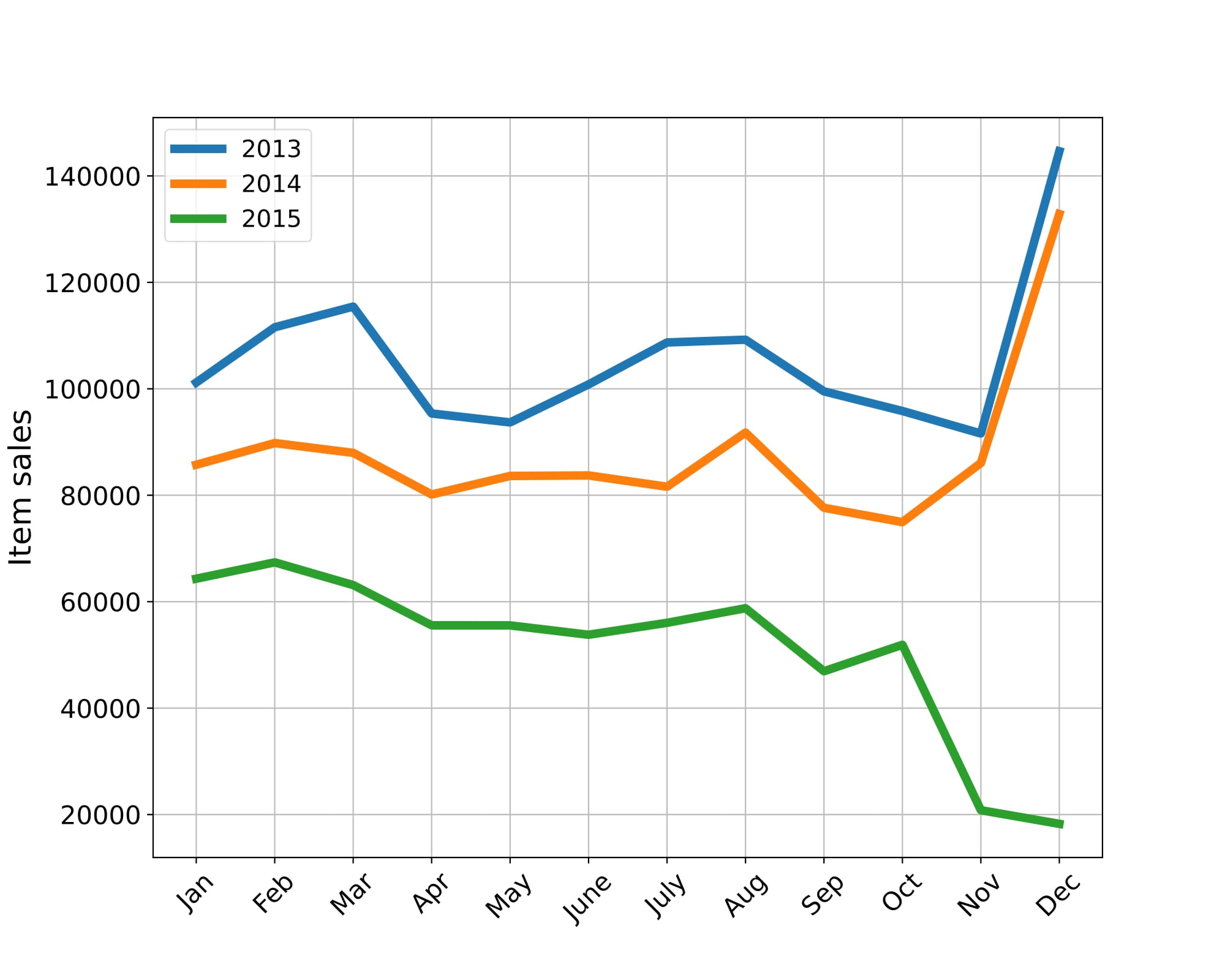
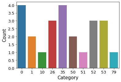
Before generating the predictions, we performed EDA on the dataset to understand the distribution of the data and identify any outliers. We also created several plots to visualize the data. The plots below show the total sales per month and the number of items per category.
For the preprocessing of the data, we decided to use the last available month (October 2015) as our validation set, to make sure that our model generalizes well to unseen data. We created two different training sets, one with the date_block_num, shop_id, and item_id, and another one that also included the item_category_id, item_maincategory_id, and item_subcategory_id (extended version). For the main and subcategories, we used the LabelEncoder to generate integers that will act as a unique identifier of each of the two names of the item’s category. The Y train includes the values of item_cnt_month, which is the goal of the prediction. These values are clipped between 0 and 20 to remove the outliers and give us better results in our predictions.
The models were trained using the training set and validated using the validation set. For the XGB we could also plot the feature importance, which is shown in the figure below.


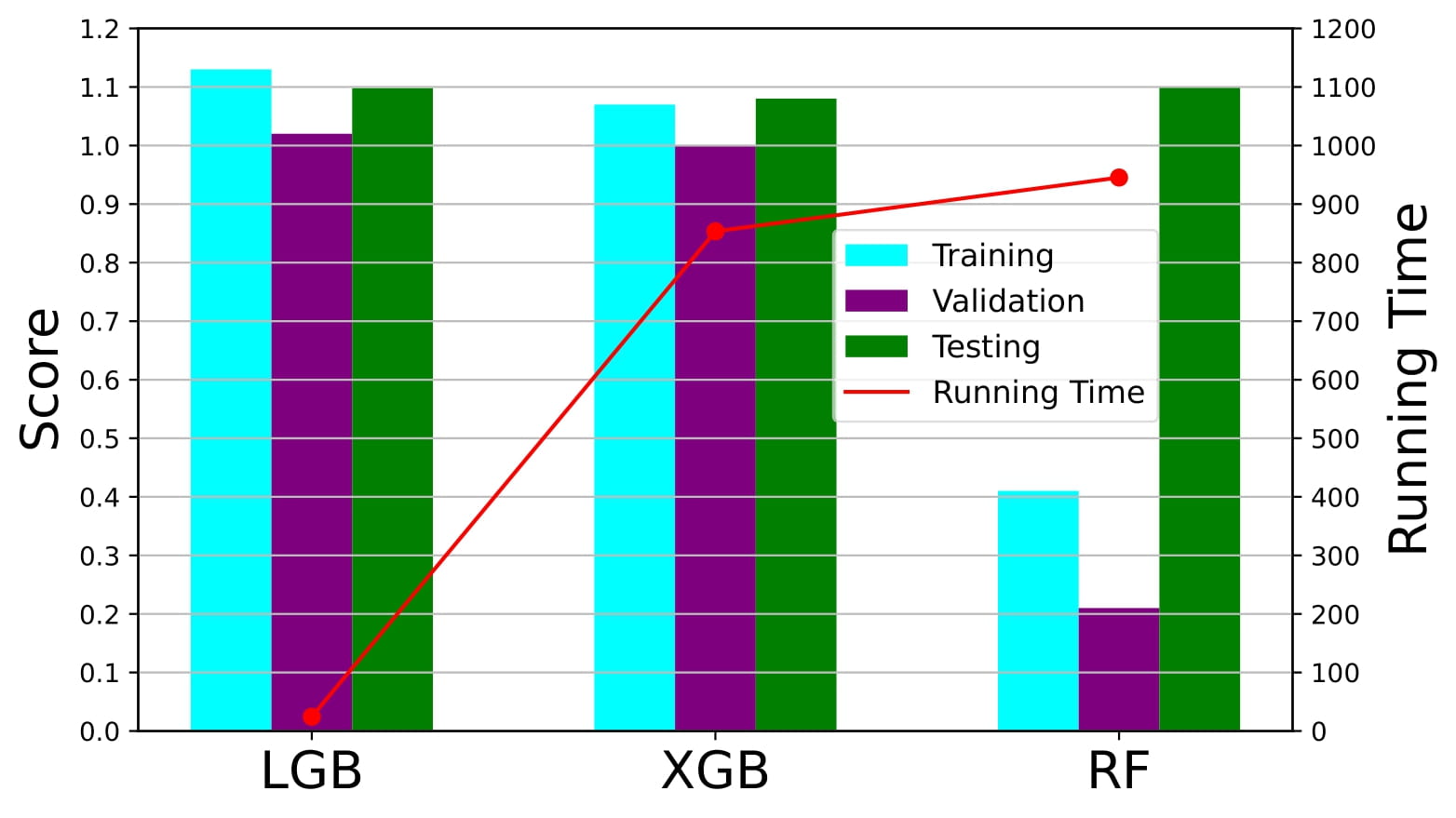
We used the RMSE as the evaluation metric to compare the performance of the models. The results of the models, for the extended version, on the training, validation, and test sets, as well as the training time, are shown in the figure below.
All the results can be summarized in the table below:
| Model | RMSE Train | RMSE Validation | RMSE Test | Training Time (s) |
|---|---|---|---|---|
| LGB | 1.39 | 1.24 | 1.19 | 20.56 |
| LGB Extended | 1.13 | 1.02 | 1.098 | 24.39 |
| XGB | 1.18 | 1.11 | 1.180 | 705.53 |
| XGB Extended | 1.07 | 1.00 | 1.080 | 853.44 |
| Random Forest | - | - | 1.119 | 678.73 |
| Random Forest Extended | - | - | 1.099 | 945.32 |
The final predictions were submitted to the Kaggle competition (RMSE test column) and the best model was the XGB for the extended version. For all the models the extended version performed better than the main version, which shows that the additional features were useful for the predictions. The feature importance plots also showed that the additional features were important for the predictions. The LGB and the Random Forest models had very similar performance, with the LGB being much faster to train, making the Random Forest model less attractive. The XGB model was the best in terms of performance, but it was also slow to train (a bit faster than the Random Forest).
In conclusion, this assignment was a great opportunity to learn about time series forecasting and implement several models to predict future sales. We were able to preprocess the data, train the models, and evaluate their performance. The results were very informative and helped us understand the strengths and weaknesses of each model. For more details, you can check the full report here. The full code can be found on my GitHub repository.