Deep Learning
projects from the course 'Deep Learning' at Leiden University
Cover Image by Growtika on Unsplash
The code for all the projects can be found in my GitHub repository. The two reports for the assignments can be found here and here.
Data Dimensionality - Distance Based Classification
In this assignment, we explored the MNIST dataset and applied dimensionality reduction techniques to visualize the data. The dataset consists of 2707 images (1707 for training and 1000 for testing) of handwritten digits from 0 to 9. The images are 16x16 pixels in size and are represented as a vector of 256 features. Each sample is labeled with the corresponding digit.
The first step was to calculate the average digit for each class in the dataset. The average digits are shown in the figure below.
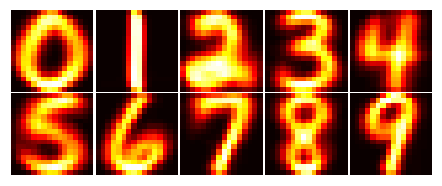
We can alo calculate the centre for each digit class and use it as a reference point for the distance-based classification. One measure of how easy is to separate two different digits is the distance between their centres. The distances can be seen in the table below.
| 0 | 1 | 2 | 3 | 4 | 5 | 6 | 7 | 8 | 9 | |
|---|---|---|---|---|---|---|---|---|---|---|
| 0 | 0.0 | 14.4 | 9.3 | 9.1 | 10.8 | 7.5 | 8.2 | 11.9 | 9.9 | 11.5 |
| 1 | 14.4 | 0.0 | 10.1 | 11.7 | 10.2 | 11.1 | 10.6 | 10.7 | 10.1 | 9.9 |
| 2 | 9.3 | 10.1 | 0.0 | 8.2 | 7.9 | 7.9 | 7.3 | 8.9 | 7.1 | 8.9 |
| 3 | 9.1 | 11.7 | 8.2 | 0.0 | 9.1 | 6.1 | 9.3 | 8.9 | 7.0 | 8.4 |
| 4 | 10.8 | 10.2 | 7.9 | 9.1 | 0.0 | 8.0 | 8.8 | 7.6 | 7.4 | 6.0 |
| 5 | 7.5 | 11.1 | 7.9 | 6.1 | 8.0 | 0.0 | 6.7 | 9.2 | 7.0 | 8.3 |
| 6 | 8.2 | 10.6 | 7.3 | 9.3 | 8.8 | 6.7 | 0.0 | 10.9 | 8.6 | 10.4 |
| 7 | 11.9 | 10.7 | 8.9 | 8.9 | 7.6 | 9.2 | 10.9 | 0.0 | 8.5 | 5.4 |
| 8 | 9.9 | 10.1 | 7.1 | 7.0 | 7.4 | 7.0 | 8.6 | 8.5 | 0.0 | 6.4 |
| 9 | 11.5 | 9.9 | 8.9 | 8.4 | 6.0 | 8.3 | 10.4 | 5.4 | 6.4 | 0.0 |
We can see that the distance between the digits is not uniform, which means that some digits are easier to separate than others. The pair of digits with the smallest distance is 7 and 9, which means that those two digits are the hardest to separate in a distance-based classification.
The next step was to apply dimensionality reduction techniques to visualize the data. We used Principal Component Analysis (PCA), t-Distributed Stochastic Neighbor Embedding (t-SNE), and Uniform Manifold Approximation and Projection (UMAP) to reduce the dimensionality of the data to 2D. The results are shown in the figure below.
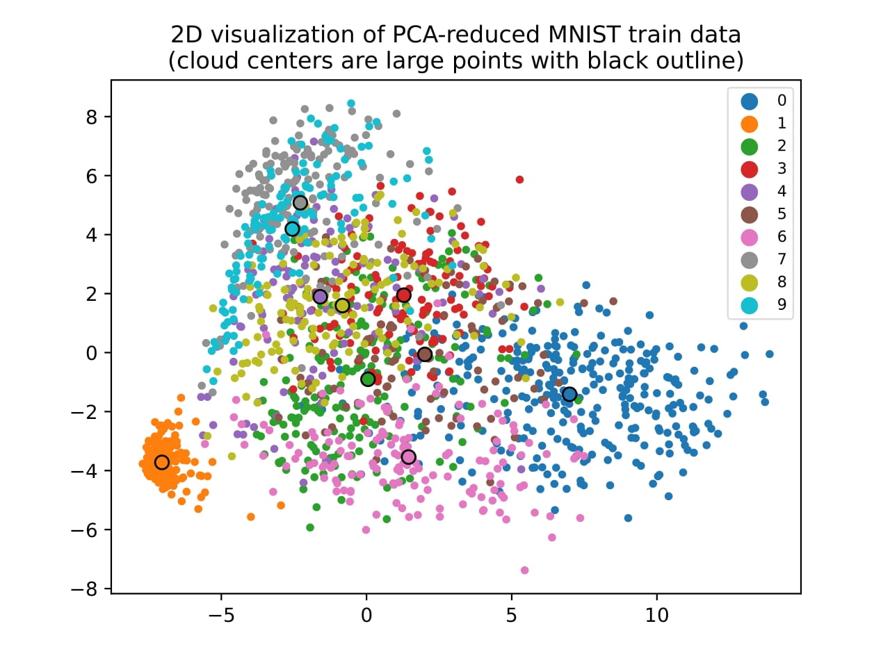
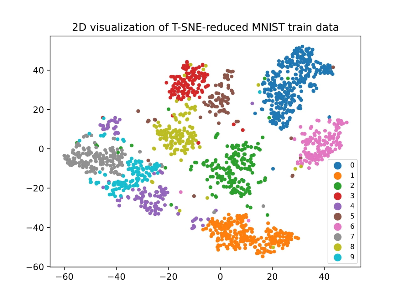
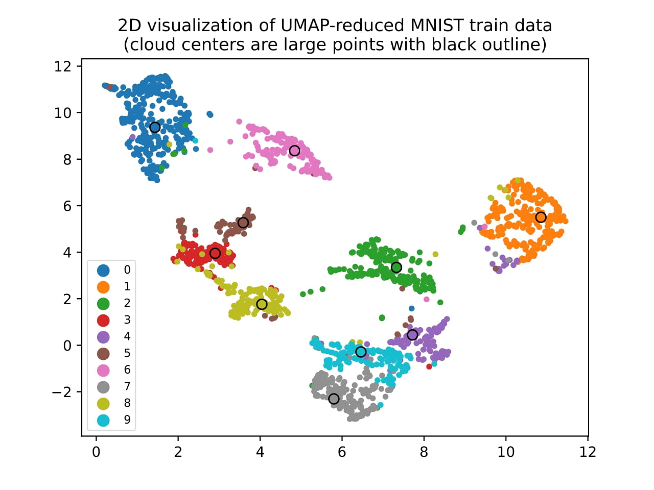
We can see that the different digits are separated in the 2D space, which means that the dimensionality reduction techniques were able to capture the underlying structure of the data. As we can see, the distances we calculated earlier are reflected in the 2D space, with some digits being closer to each other than others.
We applied two classification algorithms to the reduced data: a simple distance-based classifier, where we assigned the label of the closest centre, and a k-Nearest Neighbors (k-NN) classifier, where we assigned the label based on the majority vote of the k closest neighbours. We only tested \(k=3\) for the k-NN classifier. The results are shown in the table below.
| Classifier | Dataset | Correct | Incorrect | Accuracy |
|---|---|---|---|---|
| Distance | Train | 1474 | 233 | 86.35% |
| Test | 804 | 196 | 80.40% | |
| k-NN | Train | 1671 | 36 | 97.89% |
| Test | 914 | 86 | 91.40% |
We can see that the k-NN classifier outperformed the distance-based classifier on both the training and test datasets.
MultiClass Perceptron
For this assignment, we implemented a multi-class perceptron model to classify the MNIST dataset. The implementation was done from scratch in Python using only the numpy library (no deep learning frameworks were used).
We used two different techniques to train the model: giving the model all the training data at once (batch training) and giving the model one sample at a time (online training). The results are shown in the figure below.
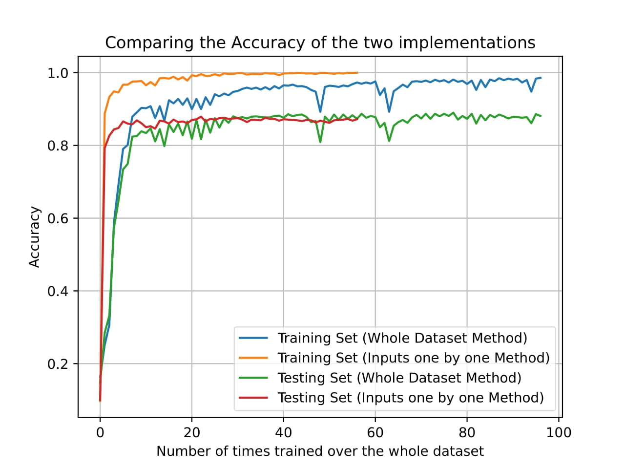
Training the model with the whole dataset at once required more epochs to converge compared to training the model one sample at a time. However, the training time was significantly shorter for the batch training method. The accuracies of the two methods can be seen in the table below.
| Method | Dataset | Correct | Incorrect | Accuracy |
|---|---|---|---|---|
| Batch | Train | 1683 | 24 | 98.59% |
| Test | 881 | 119 | 88.10% | |
| Online | Train | 1707 | 0 | 100.00% |
| Test | 872 | 128 | 87.20% |
We can see that the online training method achieved a higher accuracy on the training dataset compared to the batch training method. However, the test accuracy was slightly lower for the online training method. This can be caused by overfitting to the training data when training the model one sample at a time. On the test dataset, both methods achieved similar accuracies, with the batch training method slightly outperforming the online training method.
XOR Network - Gradient Descent
We implemented a simple neural network to solve the XOR problem using gradient descent. The XOR problem is a classic example of a non-linearly separable problem that cannot be solved by a single perceptron. The XOR takes as input two binary values (0 or 1) and outputs 1 if the inputs are different and 0 if the inputs are the same.
In our implementation, we used a neural network with one hidden layer and one output layer. The hidden layer has three neurons, and the output layer has one neuron. We trained the network using gradient descent and the backpropagation algorithm. We tested three different learning rates: 0.3, 0.6, and 0.8. The results are shown in the figure below. We also tested the network with two different initializations: uniform and normal. The mean squared error (MSE) was used as the loss function. We can see the training process for the different learning rates and initializations in the figures below.
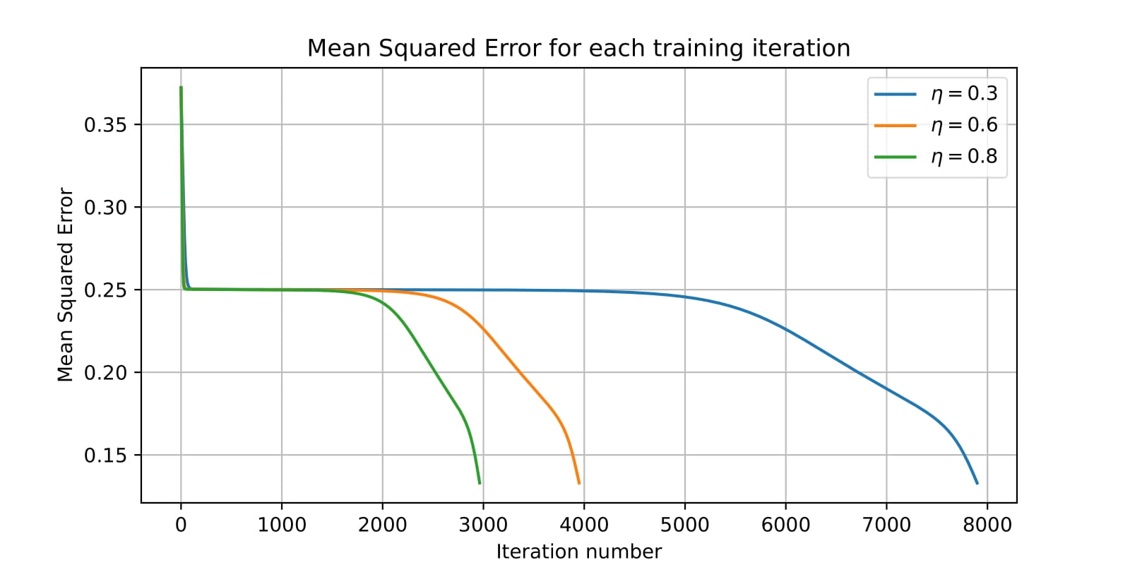
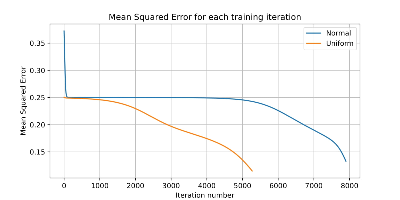
We can see that all the different strategies converged to a solution, reaching an MSE of 0, which means that the network was able to solve the XOR problem. From the diffefrent learning rates, we can see that the highest learning rate (0.8) converged faster than the other two. The uniform initialization also converged faster than the normal initialization.
We also implemented a lazy approach to the XOR problem, where we used the same network architecture but in each epoch, we randomized the weights of the network, until the network was able to solve the XOR problem. The test was to see how many epochs, on average, it took for the network to solve the XOR problem. We did four attempts with an average of 118570.75 epochs and a standard deviation of 118409.22 epochs. The results show that the network was able to solve the XOR problem, but it took a large number of epochs to do so, making it an inefficient approach.
Fashion MNIST & CIFAR 10 - TensorFlow
In this assignment, we used TensorFlow to build and train neural networks on the Fashion MNIST and CIFAR-10 datasets. The Fashion MNIST dataset consists of 70,000 grayscale images (60,000 for training and 10,000 for testing) of 28x28 pixels each, representing 10 different classes of clothing items. The CIFAR-10 dataset consists of 60,000 color images (50,000 for training and 10,000 for testing) of 32x32x3 pixels each, representing 10 different classes of objects.
We built two different neural network architectures. The first architecture is a multi-layer perceptron (MLP) with three hidden layers, each with 300, 100, and 10 neurons, respectively. The total number of parameters in the model is 266,610. The second architecture is a convolutional neural network (CNN) with three convolutional layers, each followed by a max-pooling layer, and two fully connected layers. The total number of parameters in the model is 1,413,834. We trained both models on the Fashion MNIST and CIFAR-10 datasets each time only changing the input layer to match the dataset. For each dataset we selected 5,000 samples from the training set to use as the validation set. The results are shown in the table below.
| Dataset | Model | Train Accuracy | Validation Accuracy | Test Accuracy |
|---|---|---|---|---|
| Fashion MNIST | MLP | 0.92 | 0.88 | 0.85 |
| CNN | 0.92 | 0.89 | 0.22 | |
| CIFAR-10 | MLP | 0.63 | 0.48 | 0.38 |
| CNN | 0.75 | 0.71 | 0.54 |
For the Fashion MNIST dataset, the MLP model achieved a test accuracy of 85%, while the CNN model had a very low test accuracy of 22%, while for the training and validation accuracy both models performed similarly. This indicates that the CNN model was overfitting the data. For the CIFAR-10 dataset, the MLP model achieved a test accuracy of 38%, while the CNN model had a test accuracy of 54%. The CNN model outperformed the MLP model on the CIFAR-10 dataset, indicating that the CNN model was able to capture the spatial features of the images better than the MLP model, which is something that was expected, since CNNs are more suitable for image classification tasks.
“Tell the Time” Network
The goal of this assignment is to develop a model that can tell the time from an image of an analog clock. The dataset consists of 18,000 images of analog clocks, each labeled with two values: the hour and the minute. The images are grayscale and have a resolution of 150x150 pixels. Each image is taken from a different angle and rotation, making the task far more challenging. The full dataset can be found here.
We used three different approaches to solve the problem:
- Regression: where we trained a neural network to predict a single output value for the hour and minute (e.g., 12:30 -> 12.5).
- Classification: where we trained a neural network to classify the hour and minute into discrete classes (we varied the number of classes from 24 to 60).
- Multi-head: where we trained a neural network with two output heads, one for the hour and one for the minute. For the hour we used classification with 12 classes (one for each hour), and for the minute we used regression.
For the accuracy measure, we used a “common sense” accuracy, which is the absolute value of the time difference between the predicted and the actual time. For example, the “common sense” difference between a “predicted” time of 11:50 and the “target” time of 0:10 is just 20 minutes and not 11 hours and 40 minutes. Minimizing this “common sense” error measure was the main objective of this assignment.
For both approaches (classification and regression), we used a neural network with three convolutional layers, each followed by a max-pooling layer, and two fully connected layers. For the regression we tested using both the mean squared error (MSE) and the “common sense” accuracy as the loss function. The results are shown in the table below.
| Approach | Loss Function / Number of Classes | Train Accuracy (minutes) | Test Accuracy (minutes) |
|---|---|---|---|
| Regression | MSE | 13.44 | 47.66 |
| “Common Sense” | 16.93 | 33.30 | |
| Classification | 24 classes | 14.62 | 24.79 |
| 48 classes | 7.09 | 22.89 | |
| 120 classes | 3.51 | 35.81 | |
| 240 classes | 1.98 | 41.15 | |
| 480 classes | 1.71 | 56.34 | |
| 720 classes | 1.53 | 83.38 | |
| Multi-head | 12 classes (hour) + MSE (minute) | 4.91 | 11.71 |
The “common sense” accuracy improved the test accuracy of the regression approach, indicating that it is a better loss function for this task. The classification approach outperformed the regression approach, with the best classification model (48 classes) achieving a test accuracy of 22.89 minutes. The multi-head approach outperformed both the regression and classification approaches, with a test accuracy of 11.71 minutes. This indicates that the multi-head approach was able to capture the hour and minute information separately, which improved the overall accuracy of the model. It is also interesting to note how increasing the number of classes after a certain point (48 classes) did not improve the accuracy on the test set, while it kept improving the accuracy on the training set. This indicates that the model was overfitting the training data when the number of classes was too high. This is also illustrated nicely in the figure below.
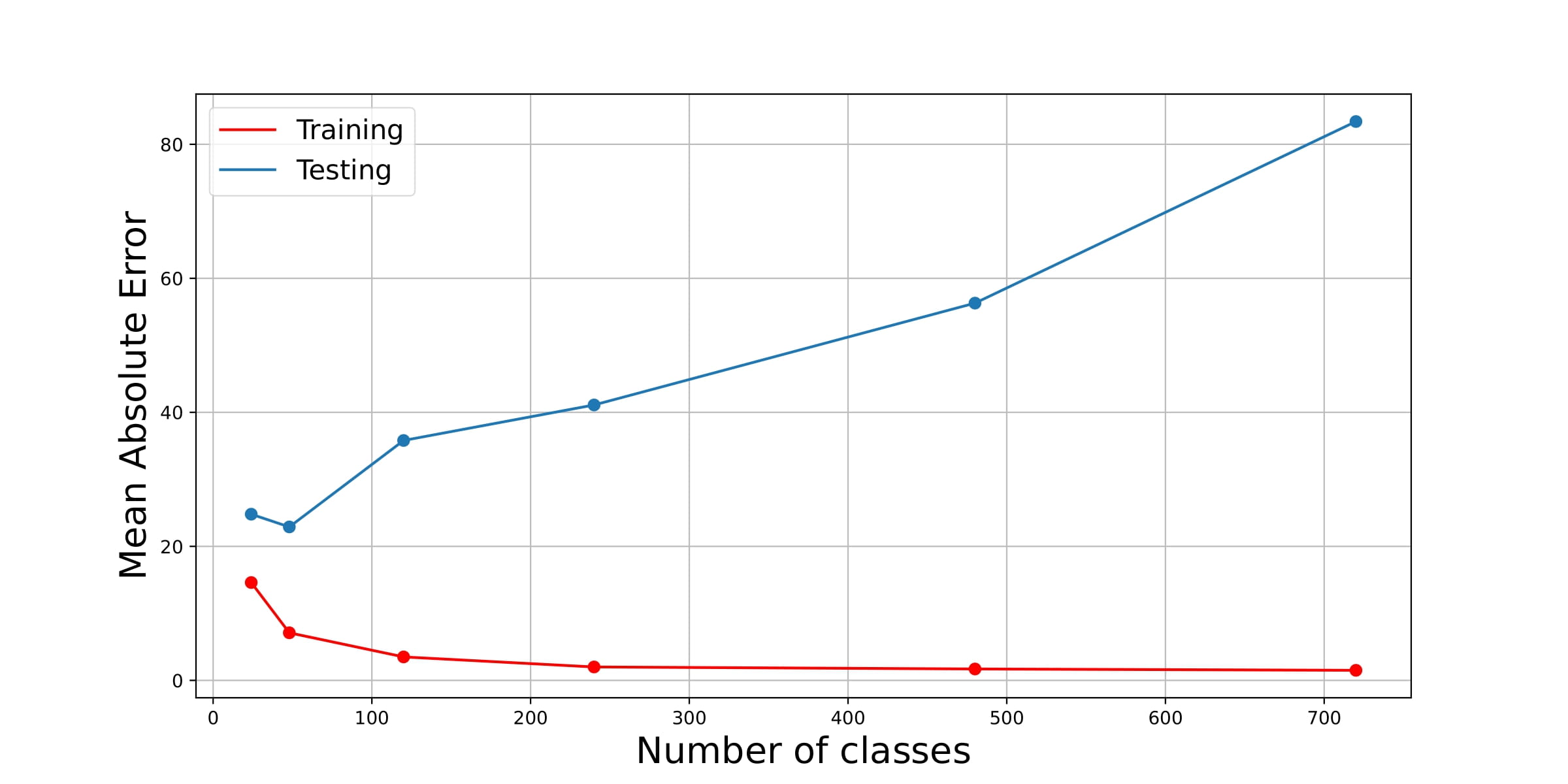
Overall, the assignment was a success, and we were able to develop a model that can tell the time from an image of an analog clock (with many different angles and rotations), with a “common sense” accuracy of 11.71 minutes on unseen data.
Generative Models - Autoencoders (VAEs) & Generative Adversarial Networks (GANs)
In this assignment, we explored generative models, specifically autoencoders (Variational Autoencoders - VAEs) and Generative Adversarial Networks (GANs). We started with a jupyter notebook that introduced the concepts of autoencoders and GANs and provided a step-by-step guide on how to implement them using TensorFlow and Keras. The notebook used a dataset of faces to train the models and generate new faces. In our approach, we used the Simpsons Faces dataset to train the models and generate new faces. The original images from the faces dataset and the Simpsons faces dataset are shown in the figure below.
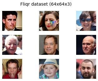
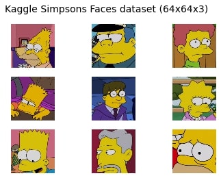
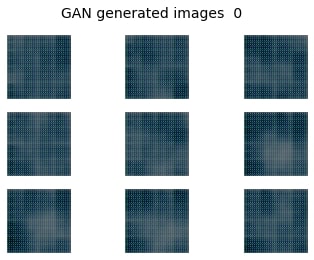
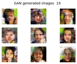
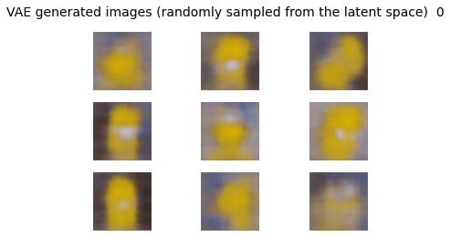
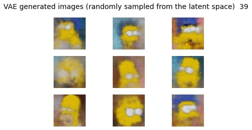
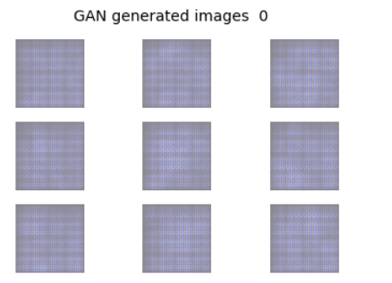
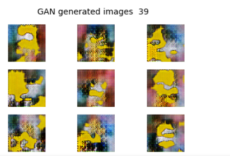
The VAE and GAN models were trained on the faces dataset and the Simpsons faces dataset. The results of the training process are shown in the figures below. We can see that the VAE model was able to generate new faces that resemble the original faces from the first epoch to the last epoch. The GAN model was also able to generate new faces, but only after a few epochs. Although the results are not perfect, we can see that the models were able to capture the underlying structure of the data and generate new faces that resemble the original faces for both datasets.
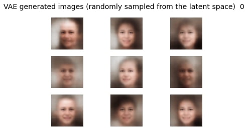
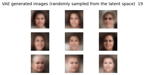
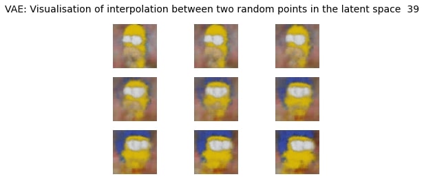
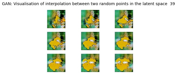
As a last step, we generated new images by interpolating between two random latent vectors in the latent space of the VAE and GAN models. The results are shown in the figures below. The results for the GAN model were not great, but we can see that the VAE model was somewhat able to generate new faces by interpolating between two random latent vectors.
Overall, the assignment was a great introduction to generative models. Although the results were not perfect, the approach that was used was very simple and only scratched the surface of what is possible with generative models.