Model-Free Reinforcement Learning for Sensorless Adaptive Optics
research project on Advanced Reinforcement Learning
This project started as part of the course “Seminar Advanced Reinforcement Learning” at Leiden University. You can find the final report here. The code is open-source and available on my GitHub repository.
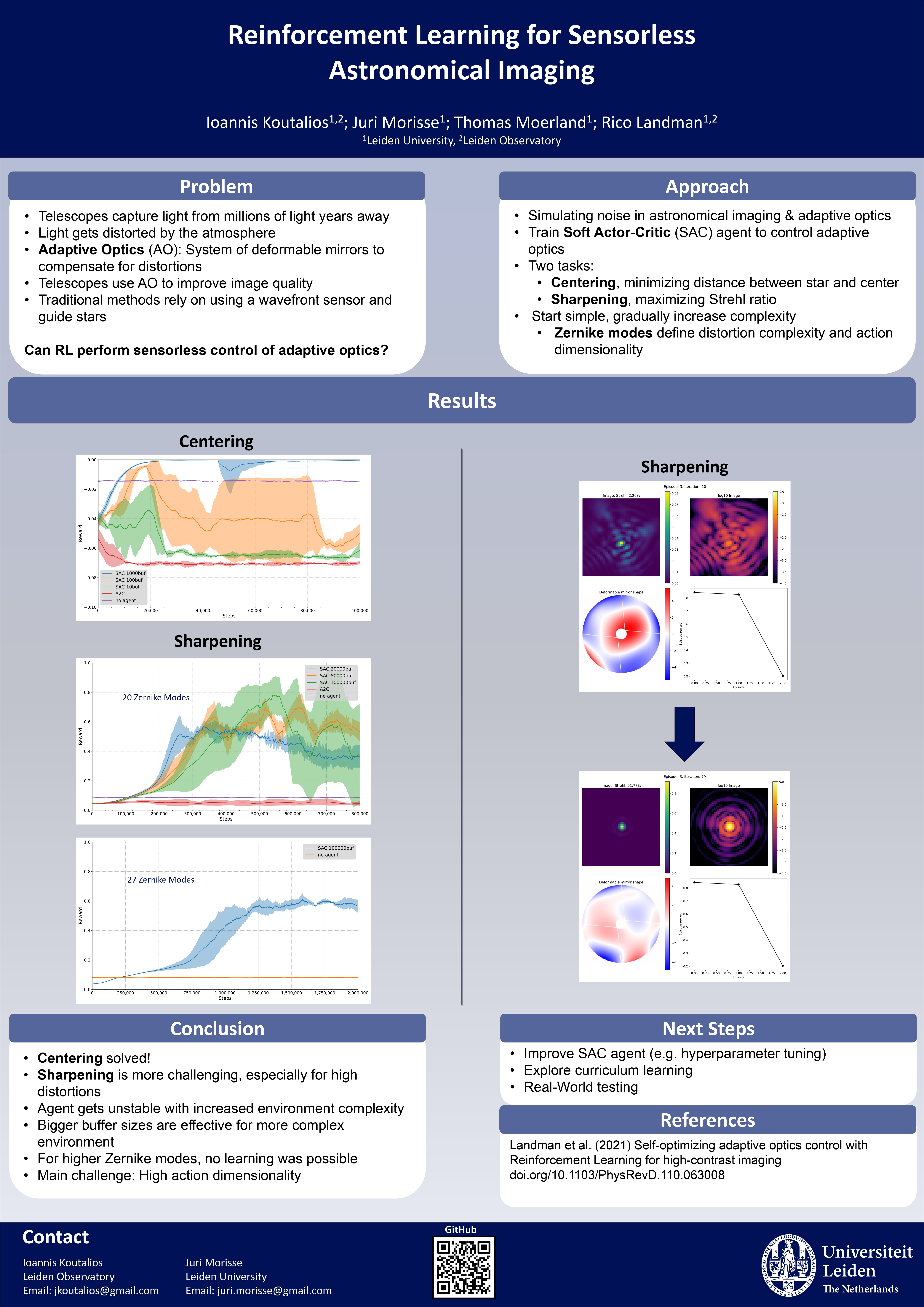
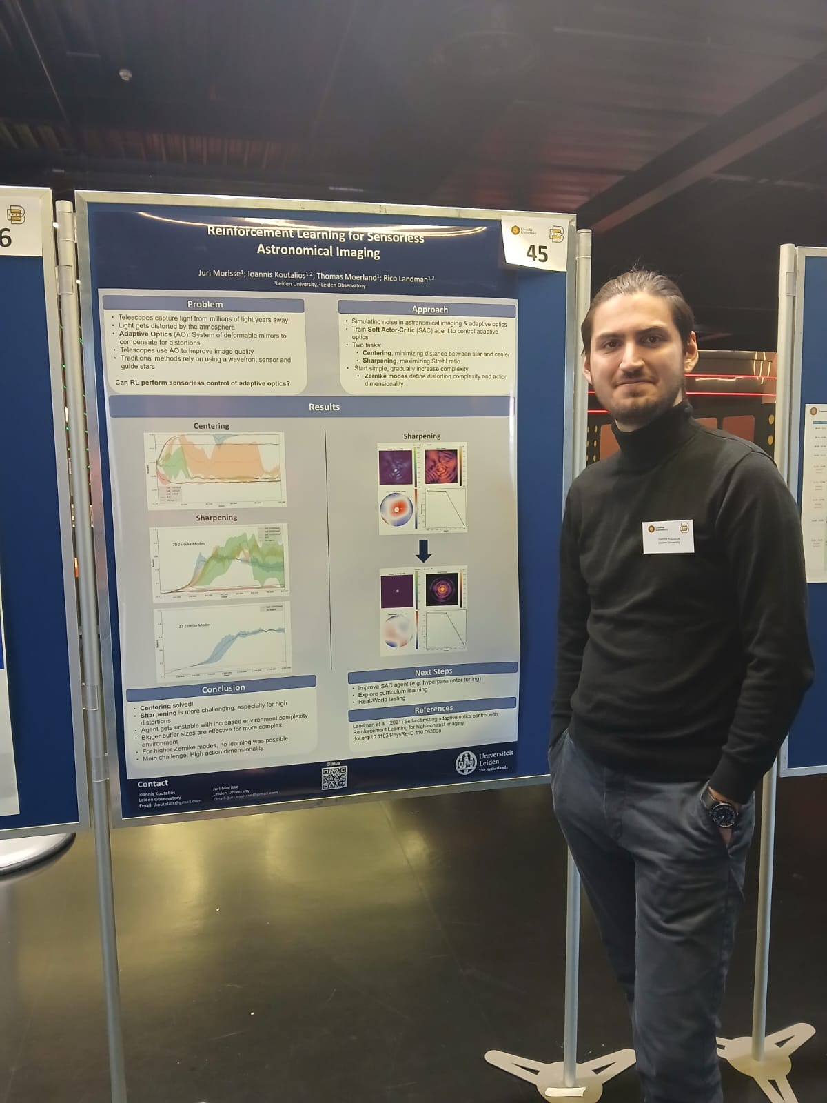
We have presented the project at the BNAIC/BeNeLearn 2024 conference with a poster. See the pictures below! You can also find the poster in pdf format.
Introduction
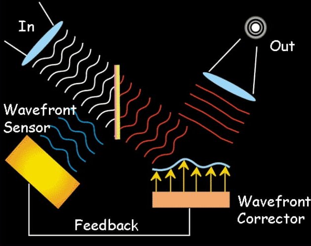
Adaptive optics (AO) is a technique used to correct for disturbances in optical systems, by adjusting a set of deformable mirrors (DM). The system consists of a wavefront sensor, a deformable mirror, and a control algorithm. The wavefront sensor measures the aberrations in the light path, the control algorithm calculates the commands to send to the deformable mirror to correct the aberrations, and the deformable mirror reshapes to correct the aberrations. Controlling a telescope’s DM is a high-dimensional decision problem that follows a constant loop of adjusting mirrors and checking the adjustment’s effect on the acquired image. Due to the sequential nature of this process and a clearly defined goal measure (reducing the noise), prior work increasingly focused on applying reinforcement learning (RL) to AO control (Durech et al., 2021; Landman et al., 2021; Nousiainen et al., 2021; Parvizi et al., 2023; Parvizi et al., 2023; Pou et al., 2022).
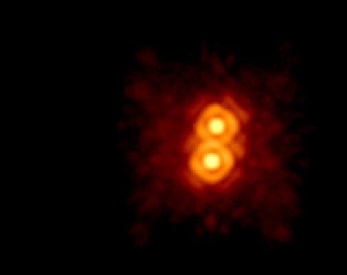
In this work, we demonstrate that RL can also be used for sensor-free AO control in the context of astronomical imaging. We argue that this approach is advantageous, as it reduces the overall system complexity by removing the sensor component and with it any potential noise or bias such a sensor can introduce.
Methodology
The number of mirrors in an AO can be high, thus creating a high-dimensional space. Atmospheric distortions can be described using a set of Zernike polynomials (Roddier, 2004). We can therefore use the same polynomials to shape the set of DM and correct aberrations. This way we are able to naturally capture the action space dimensionality (to the number of used polynomials).
We mainly use Soft Actor-Critic (SAC) from the Stable Baselines3 library, although we also experiment with the Advantage Actor-Critic (A2C) algorithm. SAC is an off-policy algorithm that uses a maximum entropy reinforcement learning framework. It is well-suited for continuous action spaces and has shown to be effective in a variety of environments. We use the implementation from the library and adapt it to our environment. Our implementation and the full paper can be accessed via GitHub.
Environments
We have used several environments to train the agents. The environments are based on the Adaptive Optics system and were created by Rico Landman. The environments are implemented in the Gym framework. You can find the original version of the environments here. The environments were adapted to work with the Stable Baselines3 library and perform the desired experiments. You can find the adapted environments here.
Image sharpening
The goal of this environment is to maximize the Strehl ratio based on focal plane images.
- Observation: The observed (noisy) image intensity in the focal plane. The image is normalized such that the values are always between 0 and 1. The image has a size of 96x96 pixels.
- Action: An array of commands to send to the actuators to reshape the deformable mirror. This is in units of radians and should have an absolute value smaller than 0.3 to avoid divergence. Default is 400 actuators.
- Reward: The Strehl ratio, which is a measure of image sharpness and is between 0 and 1.
- Things to consider:
- Partially observable Markov decision process: twin image problem (image intensity and not the electric field)
- Possible solution: provide the agent a history of observations and commands or through the use of agents that have intrinsic memory
Dark hole (not yet used in the experiments)
The goal of this environment is to remove starlight from a small region if the image.
- Observation: A measurement with information about the electric field in the dark hole region. The shape is N_probes x N_pixels, default is 5 x 499.
- Action: An array of commands to send to the actuators to reshape the deformable mirror. This is in units of radians and should have an absolute value smaller than 0.3 to avoid divergence. Default is 400 actuators.
- Reward: The log of the contrast (mean of the image intensity in the dark hole region divided by the peak intensity of the starlight).
Image sharpening easy
The goal of this environment is to maximize the Strehl ratio based on focal plane images like in the image sharpening environment. The difference is that the aberrations from the atmosphere can always be corrected by the zernike modes of the deformable mirror.
- Observation: The observed (noisy) image intensity in the focal plane. The image is normalized such that the values are always between 0 and 1. The image has a size of 96x96 pixels.
- Action: An array of commands to send to the actuators to reshape the deformable mirror. This is in units of radians and should have an absolute value smaller than 0.3 to avoid divergence. Default is with 20 modes of zernike.
- Reward: The Strehl ratio, which is a measure of image sharpness and is between 0 and 1.
Image centering
The goal of this environment is to minimize the distance between the center of the image and the center of the focal plane.
- Observation: The observed (noisy) image intensity in the focal plane. The image is normalized such that the values are always between 0 and 1. The image has a size of 96x96 pixels.
- Action: An array of commands to send to the actuators to reshape the deformable mirror. This is in units of radians and should have an absolute value smaller than 0.3 to avoid divergence. For this environment we only use 2 zernike modes (tip and tilt) to correct the aberrations.
- Reward: The negative of the distance between the center of the image and the center of the focal plane.
Experiments
From the above environments, we have chosen to focus on the Centering and Image sharpening easy environments. The Image sharpening environment is a more complex version of the Image sharpening easy environment were no filtering is applied to the atmosphere distortions. The idea is to start with a simple environment and gradually increase the complexity to see how the agent performs.
The Centering environment is the simplest environment we have used. The agent has to center the image in the focal plane. The action space is 2-dimensional and the observation space is the image intensity in the focal plane. The reward function is the negative of the distance between the center of the image and the center of the focal plane. The environment is easier to solve as the action space is smaller and the observation space is simpler.
For the Image sharpening easy environment we have the focal image of the telescope as the observation space, and the reward function is a measure of image sharpness. The action space is continuous with the dimensionality depending on the number of Zernike modes used. To simplify the problem, atmosphere distortions are filtered so that they can always be described using the same number of Zernike modes that define the action dimensionality. This makes the environment harder to solve as we increase the number of Zernike modes used. Higher degrees of the polynomials produce smaller distortions, which means that after a certain point, further increasing the number of modes will not make any significant difference to the environment and the filtering will no longer play a crucial role.
Results
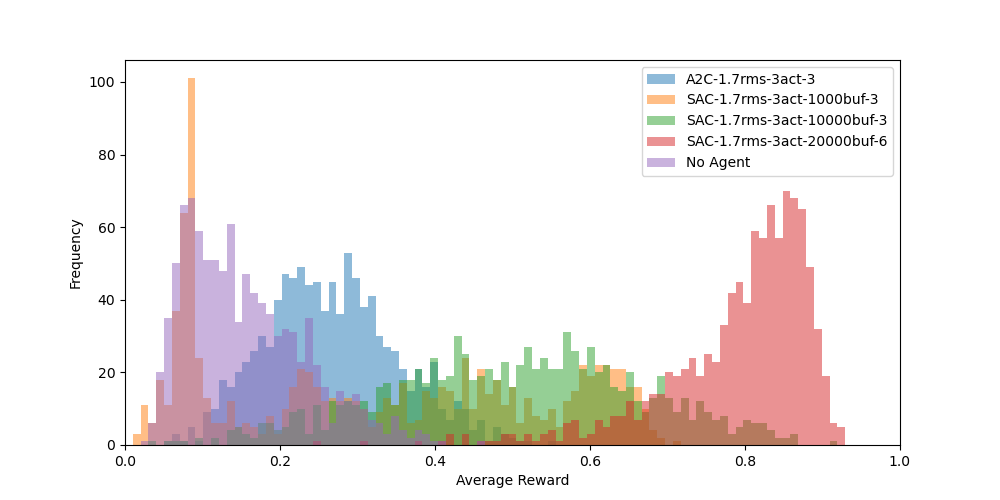
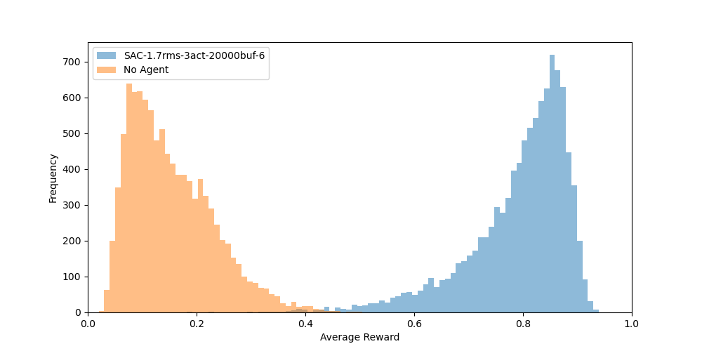
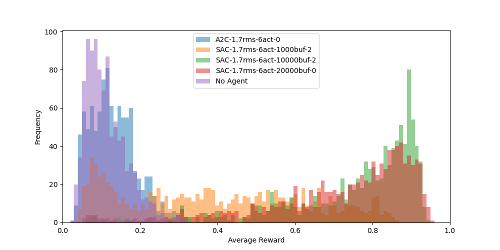
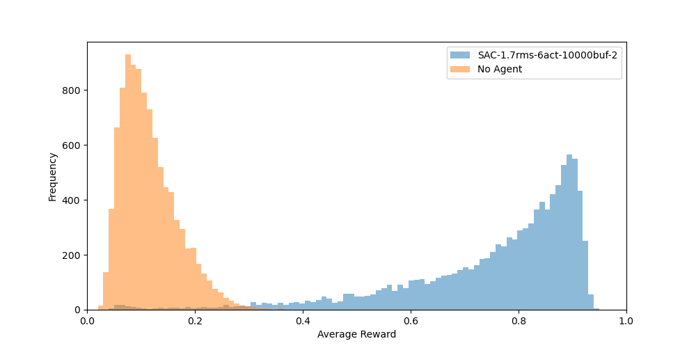
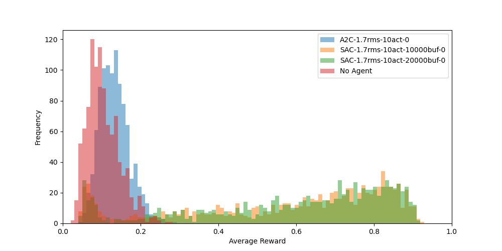
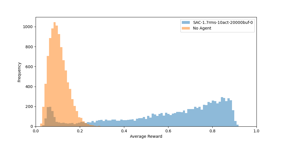
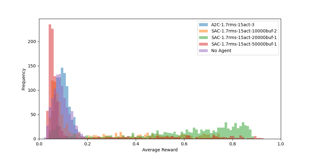
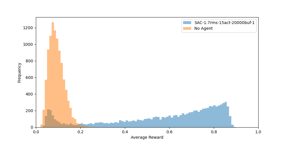
The experiments were conducted on multiple identical machines with an Intel Core i5-7500 CPU @ 3.40GHz, 8GB of RAM, and no GPU. The training was done using the Stable Baselines3 library and the models were saved using the WandB library. A different number of steps were used for each environment. We also performed an evaluation of all the agents on 1000 episodes of 100 steps and compared the results to the non-agent baseline. A second evaluation was done for the best performing agent on 10000 episodes of 100 steps. The results are presented below. For a more detailed analysis, you can check our report.
Centering
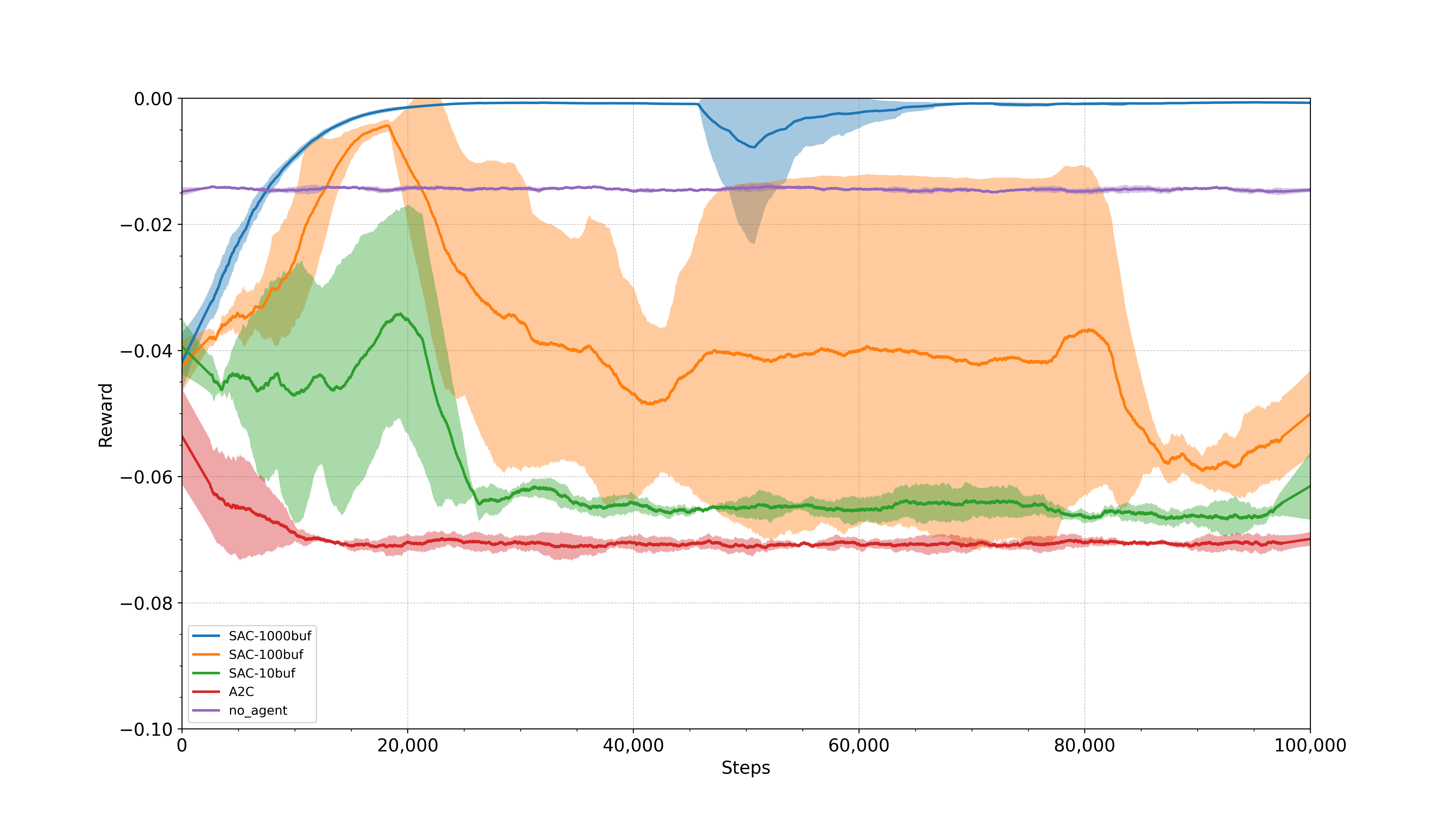
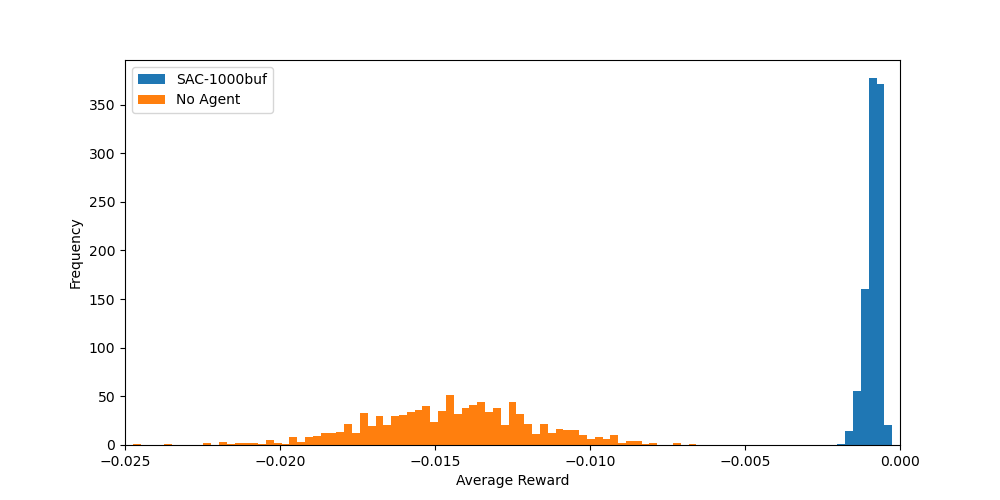
For the centering environment, we have trained agents with the SAC and A2C algorithms. The SAC algorithm with a buffer size of 1000 was able to learn a good control policy, while the A2C algorithm as well as the SAC algorithm with buffer sizes of 10 and 100 were not able to perform better than the “no-agent” baseline. The evaluation performance of the best agent, which was the SAC algorithm with a buffer size of 1000, compared to the “no-agent” baseline shows that the best agent was able to get very close to the optimal value of the reward (which is 0), while the “no-agent” baseline has a much lower performance. The learning curves and evaluation results can be found in our WandB report.
Sharpening easy
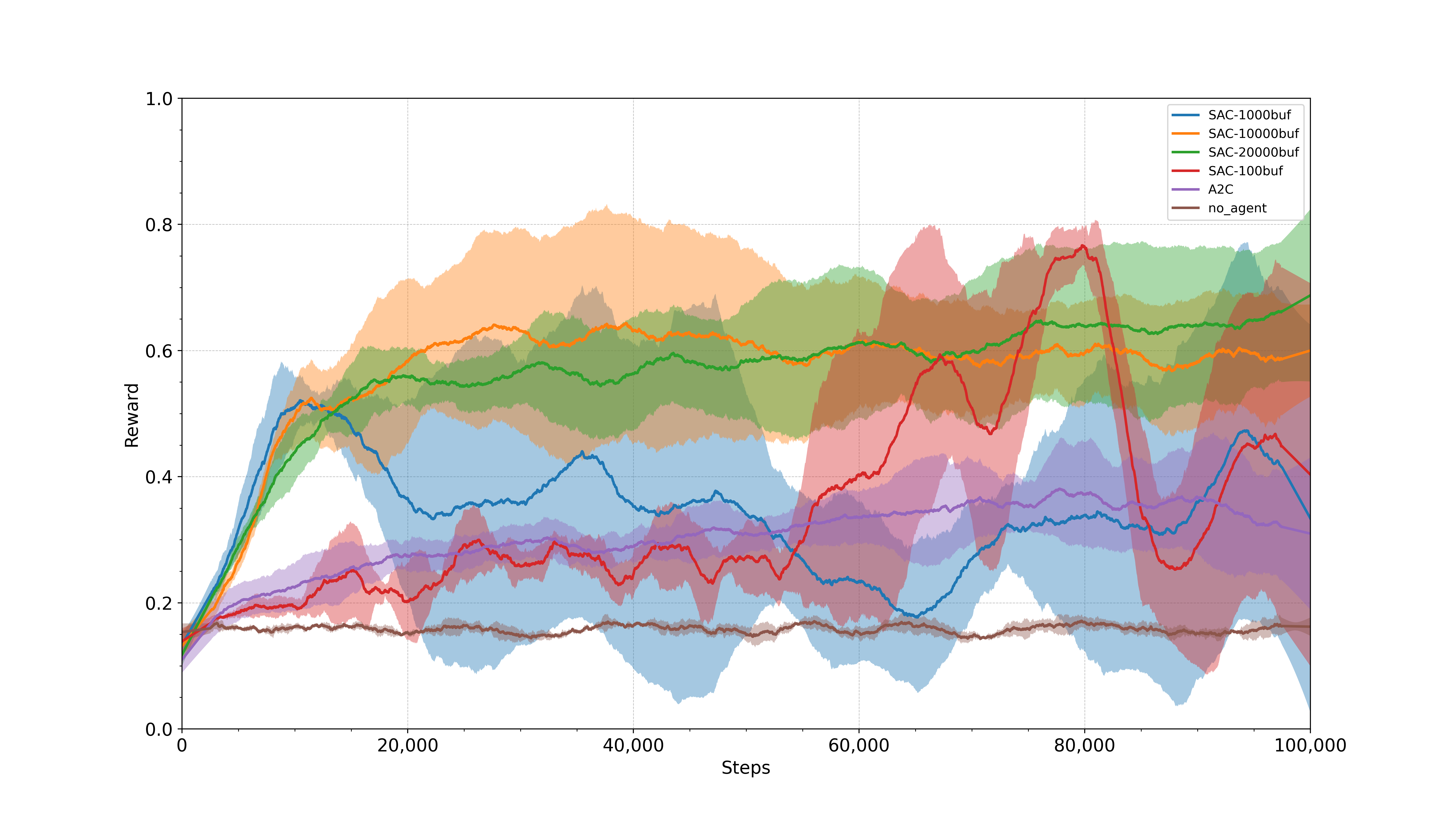
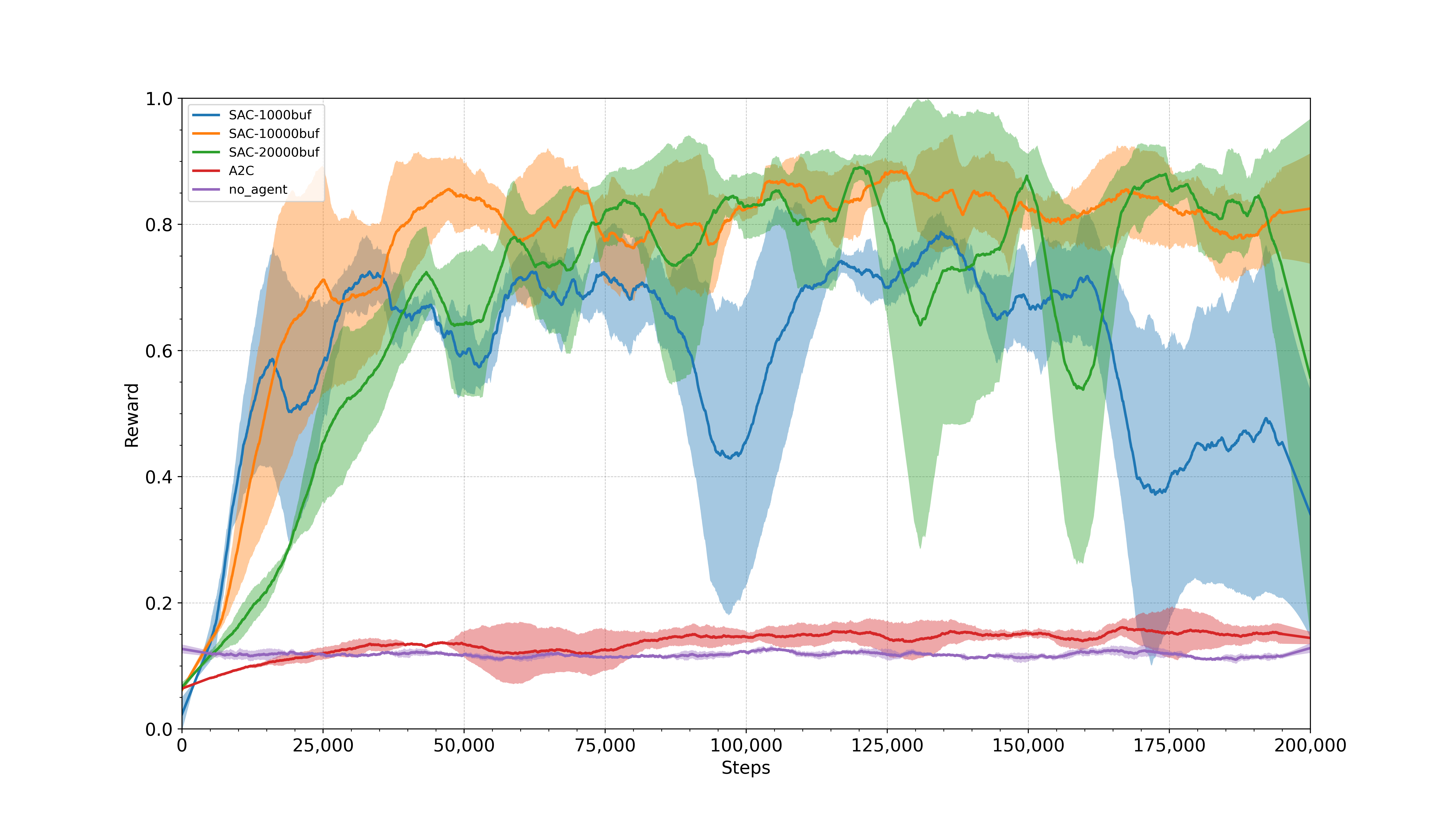
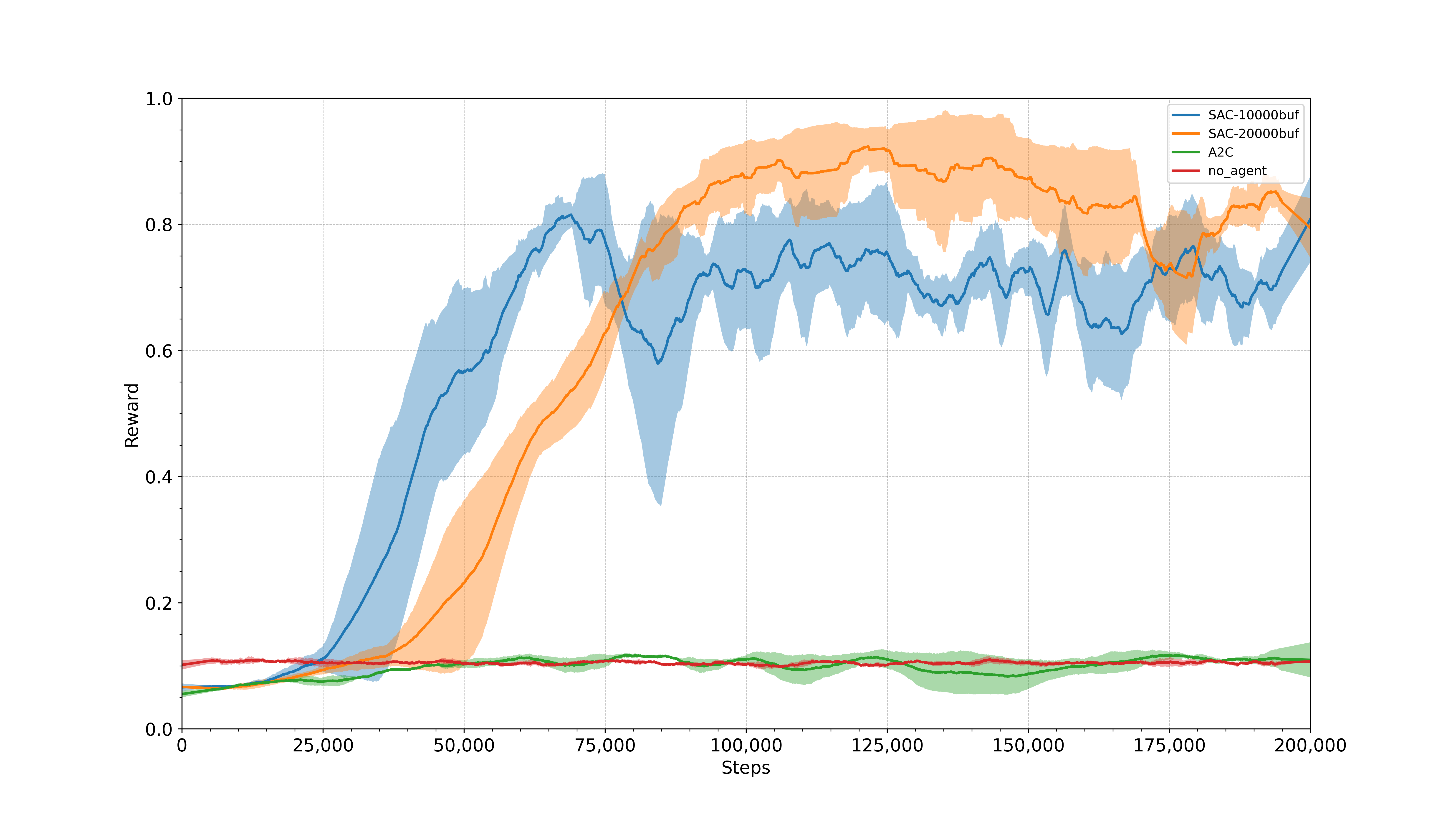
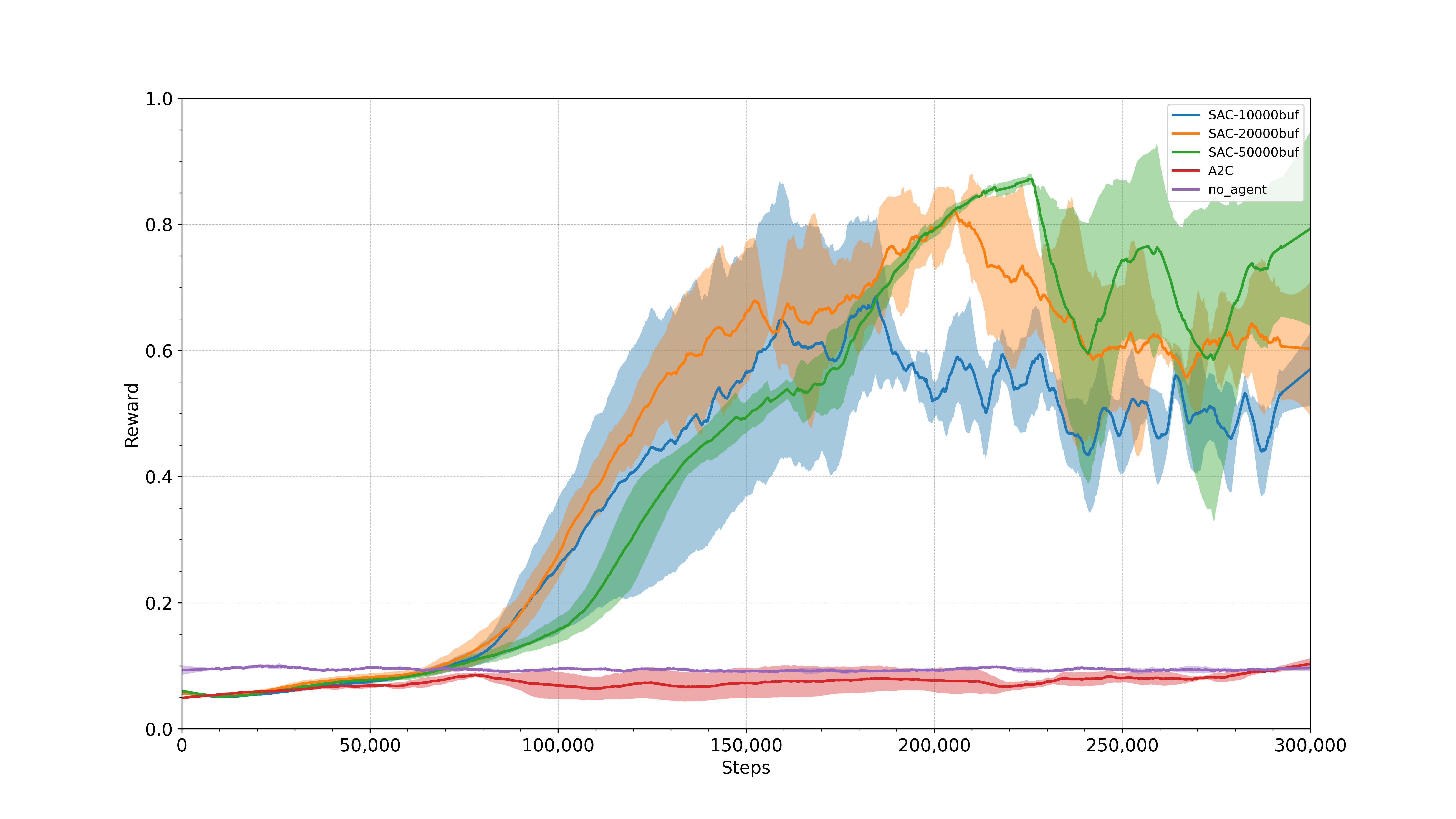
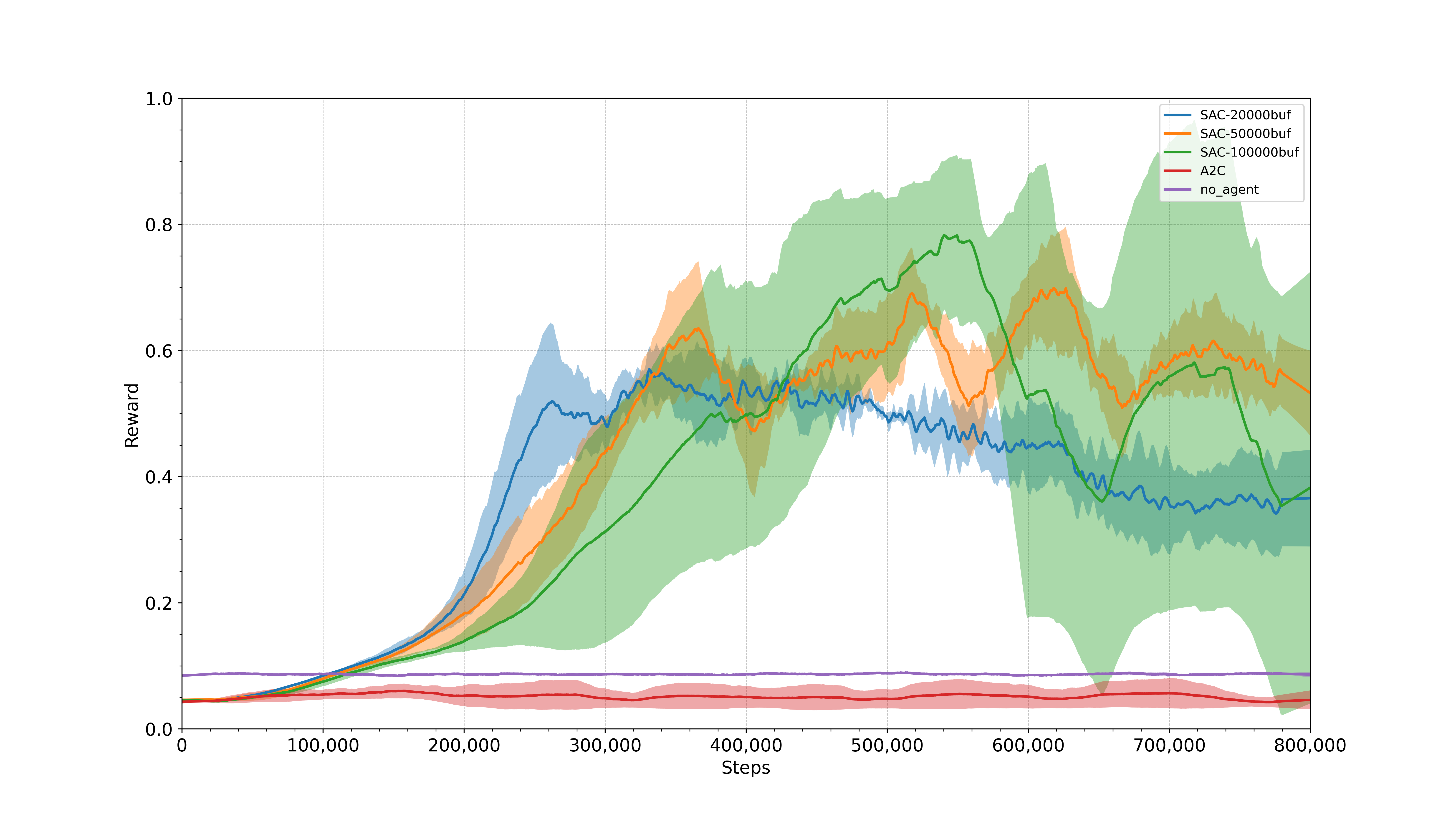
We have trained agents on the sharpening easy environment with 2, 5, 9, 14, 20, and 27 Zernike modes. Reminder that for this environment the aberrations can always be corrected by the zernike modes of the deformable mirror that we use each time. The learning curves can also be found in our WandB report.
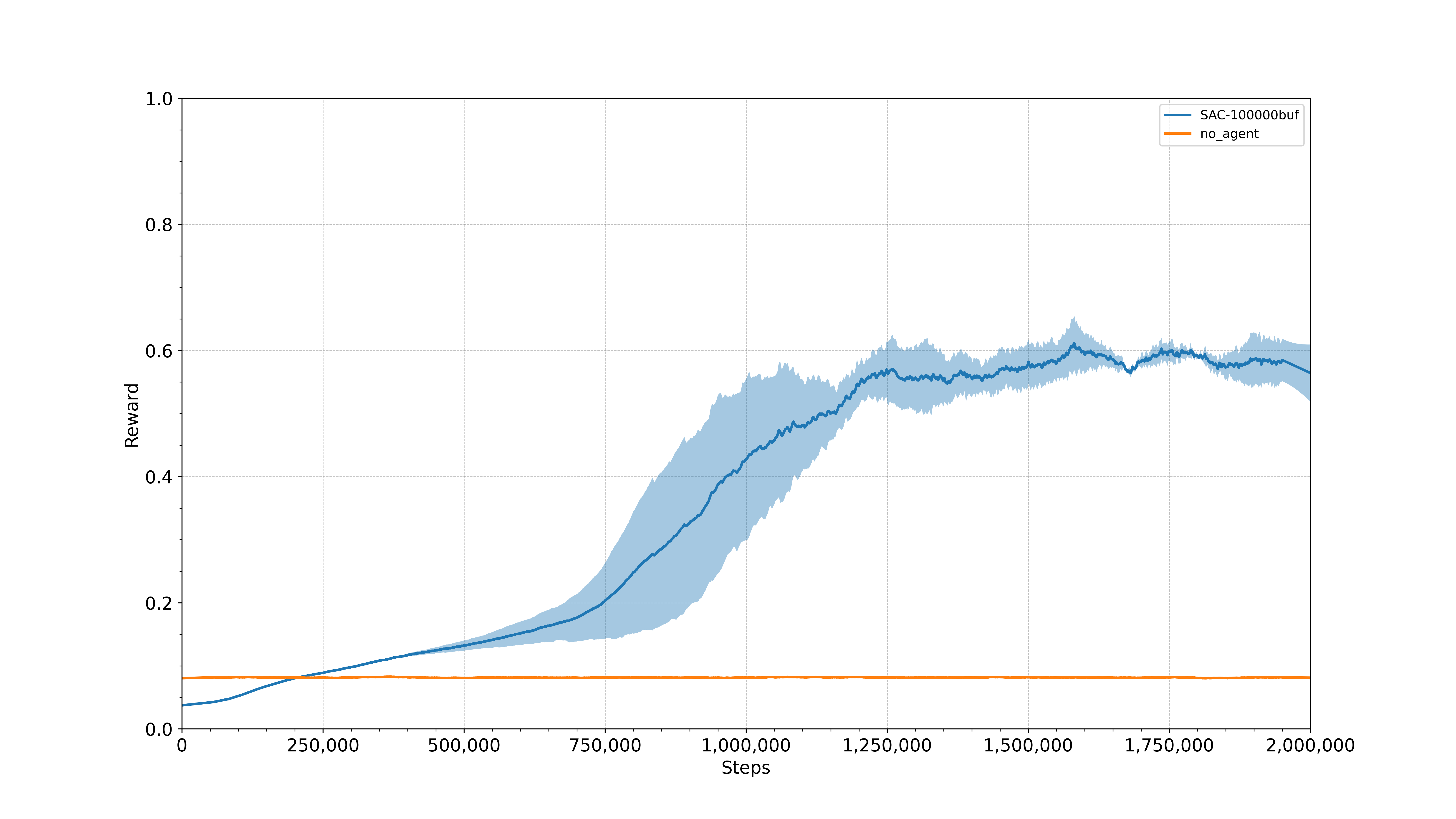
Each time we increase the number of modes, the environment gets harder to solve. For the 27 Zernike modes environment, we see that our agent is able to learn and reaches a plateau around 0.6 in the learning curve. The evaluation shows that higher performance can be achieved, there are however episodes with worse performance. The agent was also tested in the environment with a smaller number of modes and was always successful in learning a policy with an average return above \(0.6\). Above 27 Zernike modes, we were unable to see any, probably due to limitations in computational resources (e.g., buffer size and training time).
Evaluation for 2 zernike modes
Evaluation for 5 zernike modes
Evaluation for 9 zernike modes
Evaluation for 14 zernike modes
Evaluation for 20 zernike modes
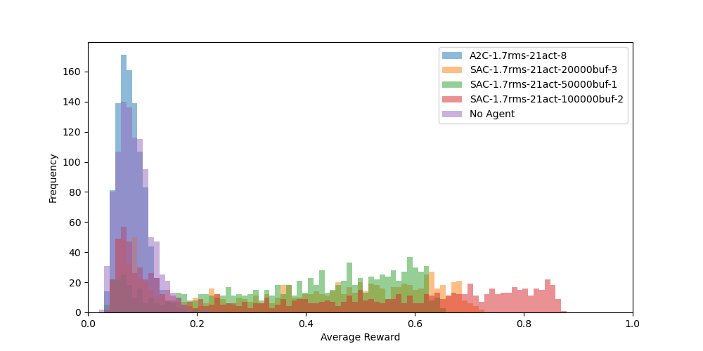
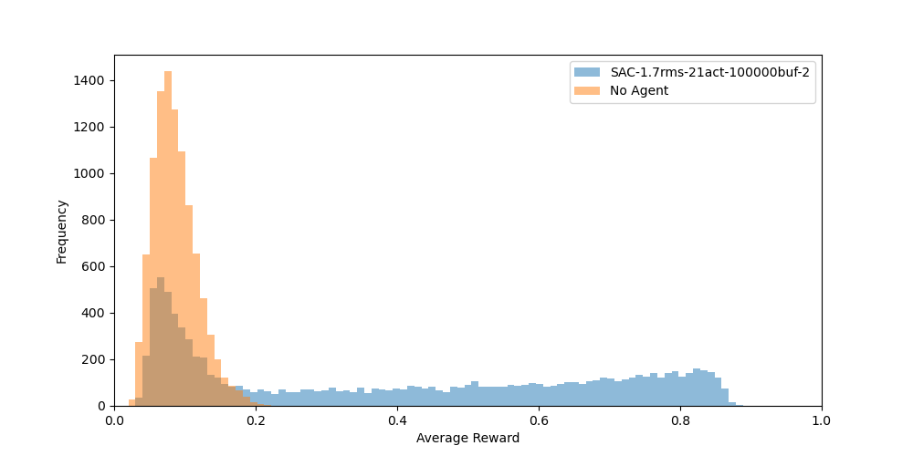
Evaluation for 27 zernike modes
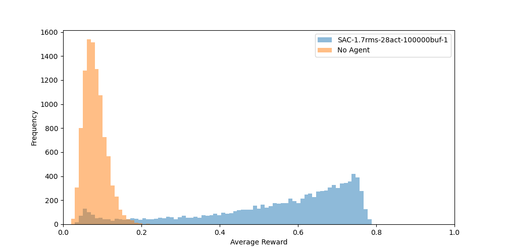
Animations
We have also created some cool animations to show the difference between the agent’s performance and the “no-agent” baseline. The animations show the agent’s performance on the Centering and Image sharpening easy environments. The animations can be found below.
Centering
Sharpening easy with 20 zernike modes
Discussion and Conclusion
This work serves as a proof-of-concept for the suitability of RL for controlling sensorless AO systems. Using an environment with controlled action dimensionality and noise, we iteratively increased complexity and achieved success for up to 27 Zernike modes. While this does not match the full complexity of real-world AO systems, it proves that RL can, in principle, effectively control sensorless AO.
We see our work as a promising first step towards RL-based AO control. Future work could build on this and, for example, explore a curriculum learning approach where an agent starts learning a simple task and gradually evolves towards solving the full task. Additionally, we see value in comparing our method to that of a sensor-based approach or testing how it performs on a real-world telescope.
References
2023
- Reinforcement Learning-based Wavefront Sensorless Adaptive Optics Approaches for Satellite-to-Ground Laser Communication2023
- Reinforcement Learning Environment for Wavefront Sensorless Adaptive Optics in Single-Mode Fiber Coupled Optical Satellite Communications DownlinksPhotonics, 2023
2022
- Adaptive optics control with multi-agent model-free reinforcement learningOpt. Express, Jan 2022
2021
- Wavefront sensor-less adaptive optics using deep reinforcement learningBiomed. Opt. Express, Sep 2021
- Self-optimizing adaptive optics control with reinforcement learning for high-contrast imagingJournal of Astronomical Telescopes, Instruments, and Systems, Sep 2021
- Adaptive optics control using model-based reinforcement learningOptics Express, Sep 2021
2004
- Adaptive Optics in AstronomySep 2004