Other Astronomical Projects
projects from various astronomical, astrophysical, and mathematical courses
Cover Image by Greg Rakozy on Unsplash
As part of my graduate and undergraduate studies, I have completed various projects as part of my coursework. In this page, I present some of the projects that I have completed in the fields of astronomy, astrophysics, and mathematics. These projects include the analysis of astronomical data, the development of computational models, and the application of mathematical techniques to solve astrophysical problems.
Matched Filtering in Gravitational Wave Data Analysis
This small project was part of the course “Astrostastistics” at the Leiden Observatory. The project consisted of implementing a matched filtering algorithm to detect gravitational wave signals in noisy data. The data used in this project were synthetic, and the templates used the approximations described by the VIRGO and LIGO collaborations (Abbott et al., 2017).
The equation of the gravitational wave signal from a binary merger was given by \begin{equation} h(t) = \frac{4A\eta M}{D} \left( \pi M f(t) \right)^{2/3} \cos\left[ \phi(t) + \phi_c \right], \label{eq:gwsignal} \end{equation} where \(A\) is a geometric prefactor (averaged over all angles making \(A = 2/5\)), \(\eta = \frac{m_1 m_2}{M^2}\) is the reduced mass, \(D\) is the luminosity distance, \(M = m_1 + m_2\) is the total mass, \(f(t)\) is the time-dependent frequency of the wave, \(\phi(t)\) is the phase of the wave, and \(\phi_c\) is a constant phase. The frequency of the wave increases with time, a phenomenon known as “chirping”. The chirp mass \(M_c\) is defined as \(M_c = \frac{(m_1 m_2)^{3/5}}{(m_1 + m_2)^{1/5}}\), and the chirpline is given by \begin{equation} f{\text{GW}}(t) = B x^{-5/8} (t_c - t)^{-3/8}, \label{eq:chirpline} \end{equation} where \(B = 16.6 \, \text{s}^{-5/8}\), \(x\) is the chirp mass in solar masses, and \(t_c\) is the moment of merger. The phase of the wave is given by \begin{equation} \phi(t) = 2\pi B x^{-5/8} (t_c - t)^{5/8}. \label{eq:phase} \end{equation} The signal shape is then given by \begin{equation} h(t) = \frac{4A\eta M \left( \pi M \right)^{2/3}}{D} \left( 16.6 x^{-\frac{5}{8}} (t_c - t)^{-\frac{3}{8}} \right)^{2/3} \cos\left[ -39.11 x^{-\frac{5}{8}} (t_c - t)^{\frac{5}{8}} + \phi_c \right]. \label{eq:gw_signal_final} \end{equation}
Equation \eqref{eq:gw_signal_final} has many parameters, some of which are degenerate. To reduce the dimensionality of the template bank, we replaced degenerate parameters with effective parameters. We can reduce the dimensionality of the template bank by considering the scale and shift symmetries of the parameters. Our model can be reduced to \begin{equation} h(t)\sim (t_c-t)^{-\frac{1}{4}}cos(-39.11x^{-\frac{5}{8}}(t_c-t)^{\frac{5}{8}}+\phi_c) \label{eq:gw_signal_final_simple} \end{equation} where \(t_c\), \(x\), and \(\phi_c\) are the only real signal parameters. In practice, when we employ matched filtering, we will shift the signal in time to match the data by varying \(t_c\), so we can argue that only \(x\) and \(\phi_c\) are the real signal parameters. The amplitude of the signal does not determine which signal is detected, but only how significantly it is detected in relation to the background noise, that is why the above equation has no amplitude parameter.
First we test the matched filtering algorithm on our own synthetic data. We create a signal, using equation \eqref{eq:gw_signal_final_simple}, and add Gaussian noise to it. We then filter the data and look for a spike in the filter output, which indicates a correlation with the signal. The results of the detection are shown in the figures below.
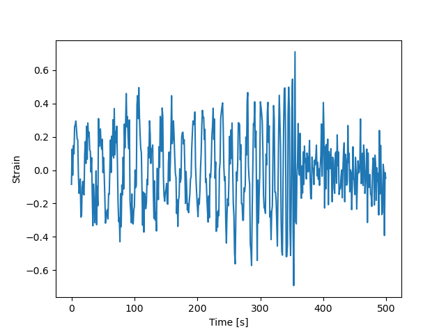
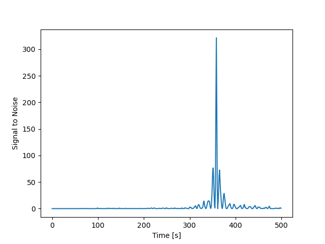
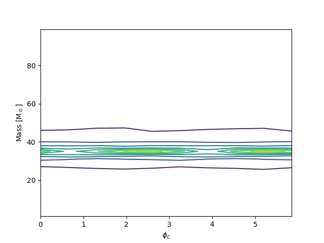
As we can see from the figures, the matched filtering algorithm is able to detect the gravitational wave signal in the synthetic data and recover the parameters we used to create the signal. Now we can tet the algorithm on the data of the exercise, which may or may not contain synthetic gravitational wave signals. We have three data streams that we need to test for gravitational wave signals. The results of the detection are shown in the figures below.
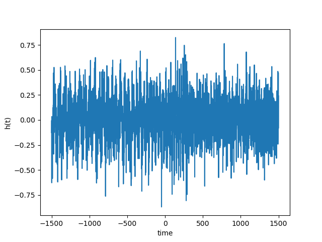
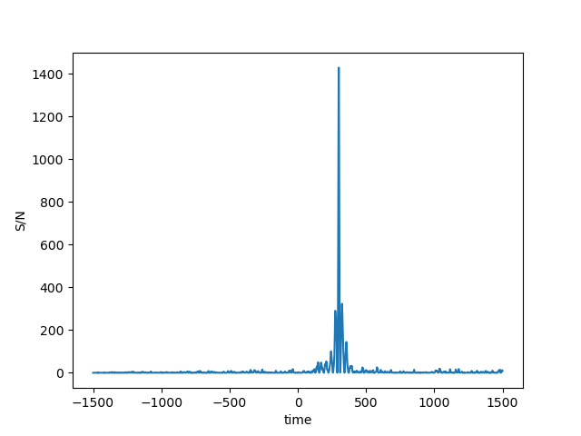
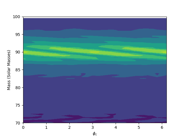
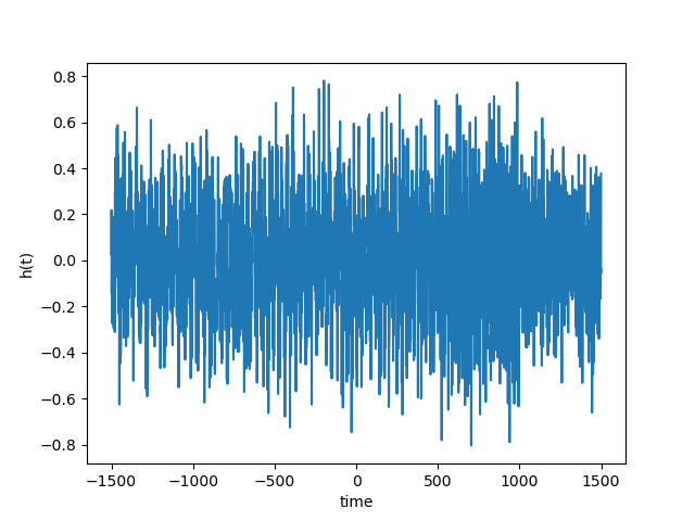
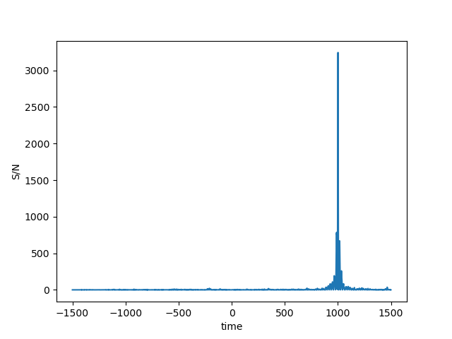
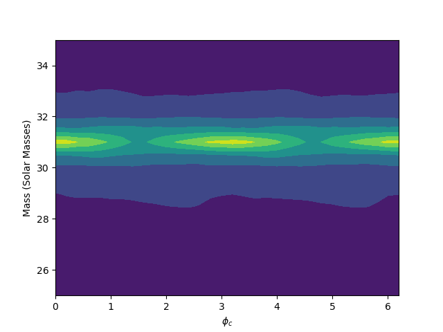
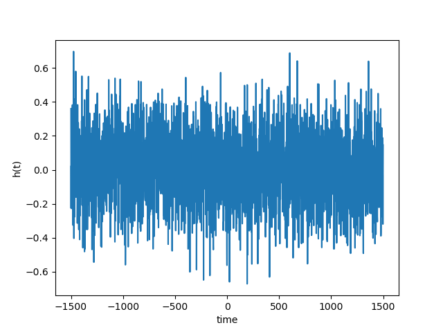
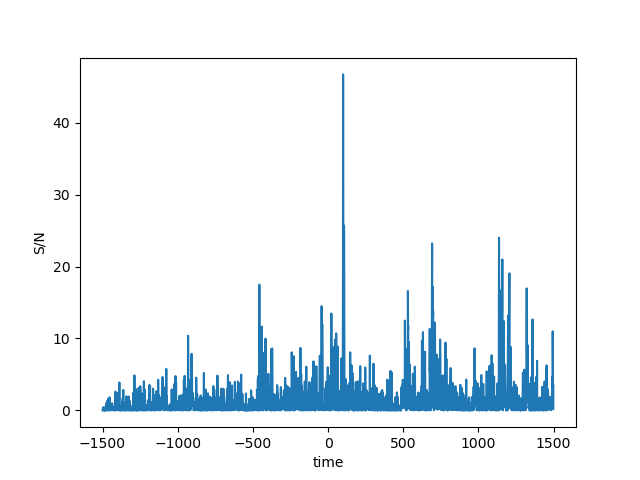
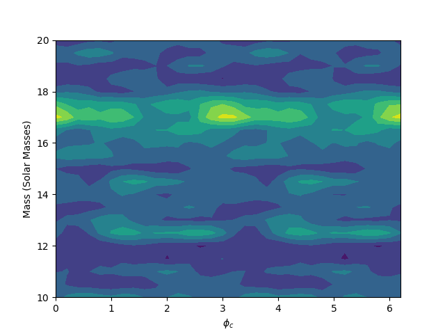
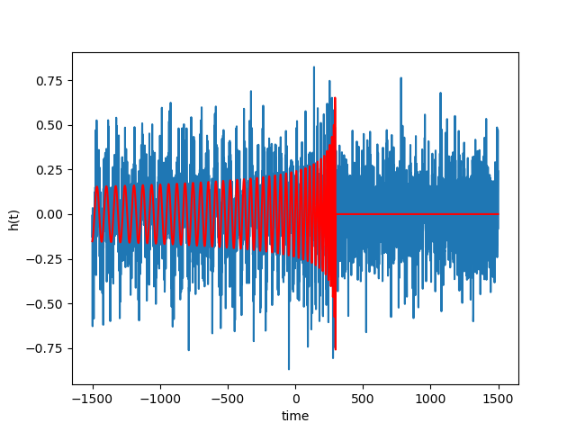
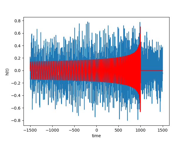
The matched filtering algorithm was able to detect the gravitational wave signals in two of the three data streams. For the third data stream, the algorithm detected a very weak signal, which was not significant enough to be considered a detection.The detected waves are shown in the figures below. The algorithm was able to recover the parameters of the signals, such as the chirp mass and the phase. The results of the detection are consistent with the parameters used to create the signals. The algorithm was not able to detect a gravitational wave signal in the third data stream, which did not contain a signal. The final results are summarized in the table below, for the code as well as instructions on how to run it, please visit the GitHub repository.
| Data Stream | Time of Merger | Chirp Mass | Phase | Detected |
|---|---|---|---|---|
| 1 | 299.0 | 90.0 | 6.2 | Yes |
| 2 | 1000.0 | 31.0 | 3.2 | Yes |
| 3 | - | - | - | No |
Stellar Structure and Evolution Lab Assignment
For the course “Stellar Structure and Evolution” at the Leiden Observatory, I completed a project on the evolution of a star from the protostar phase to the white dwarf phase. The project aimed to study the differences in the evolution of the two stars and to understand the physical processes that drive the evolution of stars. For the star evolution simulation, we used the Modules for Experiments in Stellar Astrophysics (MESA) code (Paxton et al., 2011; Paxton et al., 2013; Paxton et al., 2015; Paxton et al., 2018; Paxton et al., 2019; Jermyn et al., 2023). For more information on the MESA code, please visit the documentation on the MESA website.
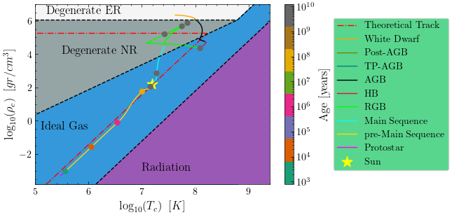
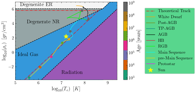
The evolution of the stars was studied by plotting the density as a function of the central temperature in a log-log plot. The different regions where each equation of state dominates were identified. We have four different equations of state:
\(P_{\text{gas}} = \frac{R}{\mu} T \rho \quad \text{(ideal gas)}, \quad P_{\text{e}} = K_{\text{NR}} \left( \frac{\rho}{\mu_e} \right)^{5/3} \quad \text{(non-relativistic degenerate electron gas)},\) \(P*{\text{e}} = K*{\text{ER}} \left( \frac{\rho}{\mu*e} \right)^{4/3} \quad \text{(extreme relativistic degenerate electron gas)}, \quad P*{\text{rad}} = \frac{a T^4}{3} \quad \text{(radiation pressure)},\)
for the different phases that a gas can have. We denote with \(P_{\text{gas}}\) the gas pressure, \(P_{\text{e}}\) the electron pressure, \(P_{\text{rad}}\) the radiation pressure, \(R\) the gas constant, \(\mu\) the mean molecular weight, \(\mu_e\) the mean molecular weight per electron, \(K_{\text{NR}}\) the non-relativistic degeneracy constant, \(K_{\text{ER}}\) the extreme relativistic degeneracy constant, \(a\) the radiation constant, and \(T\) the temperature. While stars evolve, they can go through different phases where different equations of state dominate. In the plots below, we can see the evolution of the 1 solar mass star and the 2 solar mass star and the different regions that they go through.
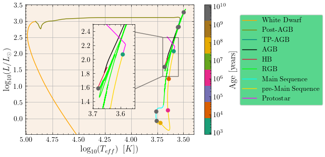
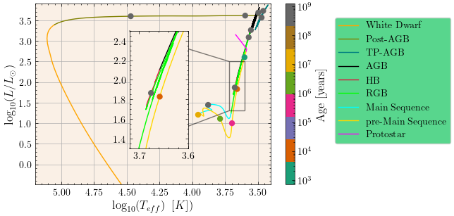
We can also see the evolution of the stars in a Hertzsprung-Russell diagram, which is a log-log plot of the luminosity as a function of the effective temperature. In a typical Hertzsprung-Russell diagram there are different regions where stars are located depending on their evolutionary stage. As stars evolve, they move through these regions, starting from the protostar phase, then the main sequence, where they spend most of their lives, and finally they go through the red giant phase, the horizontal branch and the asymptotic giant branch, to end up as white dwarfs. The Hertzsprung-Russell diagrams for the 1 solar mass star and the 2 solar mass star are shown below.
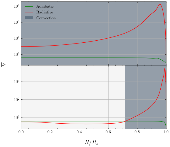
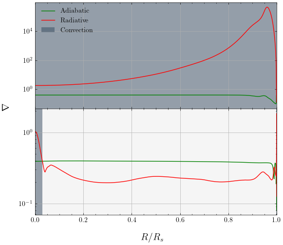
Finally, we can study the gradients of the stars as a function of the radius of the star. The gradients are important because they determine the energy transport mechanism in the star. When the adiabatic gradient is larger than the radiative gradient, the star is convective. The gradients of the 1 solar mass star and the 2 solar mass star for the pre-main sequence phase and the main sequence phase are shown below.
This project was a great opportunity to learn about the physical processes that drive the evolution of stars and to understand the different regions that stars go through as they evolve. The MESA code is a powerful tool that allows us to simulate the evolution of stars and to study the physical processes that drive their evolution. For the code as well as instructions on how to run it, please visit the GitHub repository or you can check the final report here.
MODELLING SUB-NEPTUNE MASS PLANETS INTERIOR
As part of the course “Exo-planets” at the Leiden University, I completed a project on the evolution of low-mass planets with an envelope made mostly of hydrogen and helium. The project aimed to simulate the interiors and evolution of these planets and to study how irradiation from a central star affects their structure and evolution. The project followed previous work (Chen & Rogers, 2016) and used the Modules for Experiments in Stellar Astrophysics (MESA) (Paxton et al., 2011; Paxton et al., 2013; Paxton et al., 2015; Paxton et al., 2018; Paxton et al., 2019; Jermyn et al., 2023) code to simulate the evolution of the planets.
The project started by creating a single planet with a mass of 30 Earth masses. The planet was coreless and consisted only of a mix of hydrogen and helium gas. The next step was to create a core for the planet. The core had the same composition as the Earth, which allowed us to calculate the density of the core. We created five different planets with different core masses and densities, 3, 5, 7, 10, and 12 Earth masses. After creating the core, we reduced the mass of the planets by reducing the mass of the gaseous envelope that surrounded the core. For each core mass, we created two different planets with different values for the ratio between the mass of the envelope and the total mass of the planet. The final masses of the planets are shown in the table below.
| Core Mass | fenv | Total Mass |
|---|---|---|
| 3M⊕ | 0.1 | 1.001 · 10⁻⁵M⊙ |
| 0.01 | 9.104 · 10⁻⁶M⊙ | |
| 5M⊕ | 0.1 | 1.669 · 10⁻⁵M⊙ |
| 0.01 | 1.517 · 10⁻⁵M⊙ | |
| 7M⊕ | 0.1 | 2.337 · 10⁻⁵M⊙ |
| 0.01 | 2.124 · 10⁻⁵M⊙ | |
| 10M⊕ | 0.1 | 3.338 · 10⁻⁵M⊙ |
| 0.01 | 3.035 · 10⁻⁵M⊙ | |
| 12M⊕ | 0.1 | 4.006 · 10⁻⁵M⊙ |
| 0.01 | 3.642 · 10⁻⁵M⊙ |
The next step was to add an artificial luminosity that would deposit some energy inside the planets. The result of this process was the inflation of the planets, which affected the initial entropy at the base of the gaseous envelope of each planet. The artificial luminosity that was implemented was \(L_{\text{center}} = 2 \times 10^{27} \, \text{erg/sec}\). The final step was to see how the planets evolved. During the evolution, a new more realistic luminosity was set, \(L_{\text{center}} = 5M_{\text{core}} \times 10^{-8} \, \text{erg/sec}\), where \(M_{\text{core}}\) is in units of grams. The planets were allowed to evolve for a timescale of \(5 \times 10^9\) years.


The results of the project showed that the planets evolved differently depending on their core mass and the ratio between the mass of the envelope and the total mass of the planet. For a full explanation of the results, please refer to the final report here.
The second part of the project focused on the evolution of one of the planets previously made, this time with irradiation from a central star. We started with the heaviest of the planets created in the previous work, a planet with a core mass of 12 Earth masses and an envelope mass of 0.1. We create two different scenarios with different levels of irradiation. The first scenario had an outside flux of \(10F_{\oplus}\), and the second scenario had an outside flux of \(100F_{\oplus}\). These scenarios will be compared to the original evolution of the planet with no external heating. The planets were allowed to evolve for a timescale of \(5 \times 10^9\) years (same as the previous work).
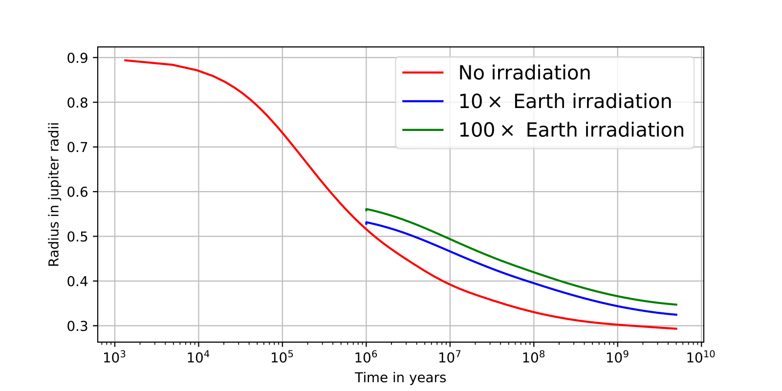
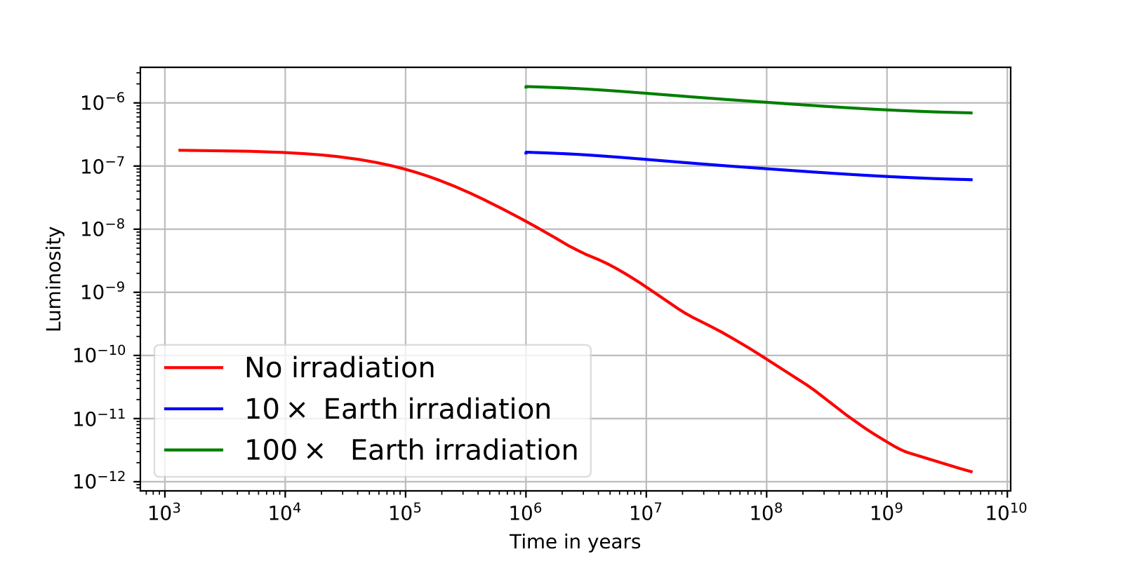
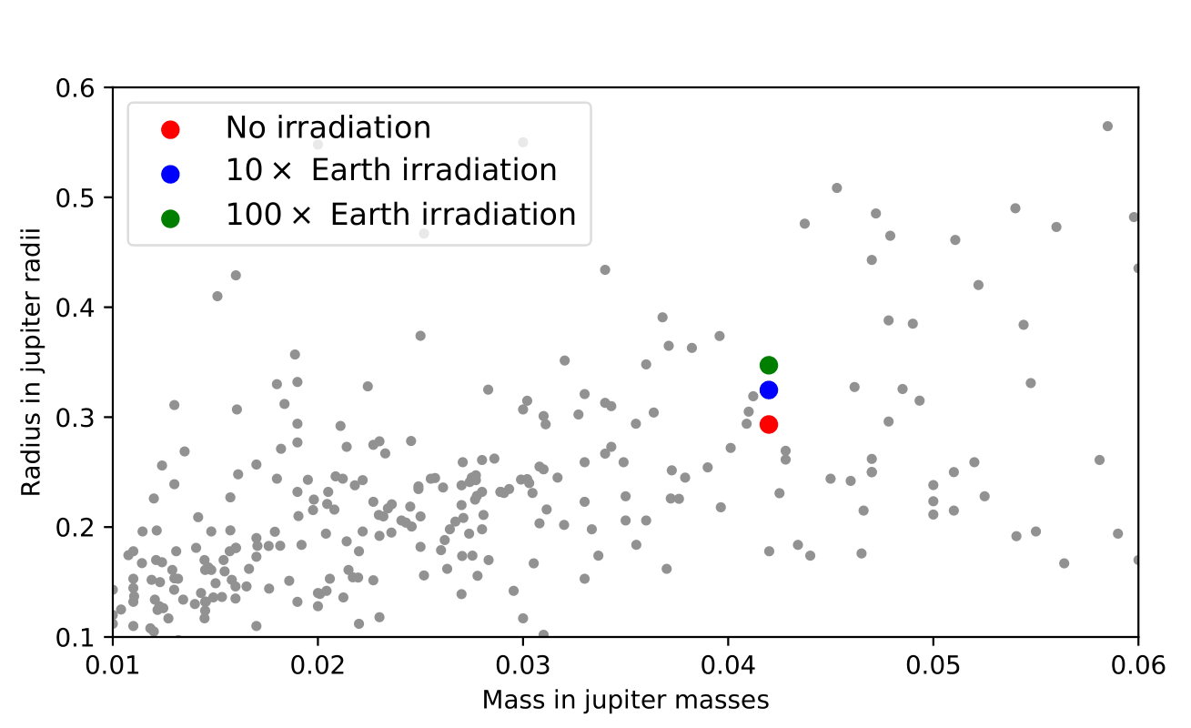

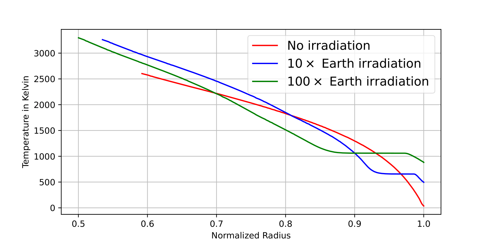
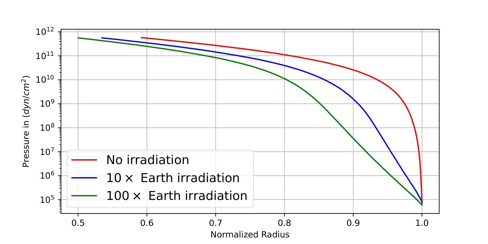
As we can see from the results, the irradiation from a central star affects the evolution of the planet. The planet with no irradiation evolves differently from the planet with irradiation, while the level of irradiation also plays a crucial role. For the full explanation of the results, please refer to the final report here.
This project was my first experience with MESA code and the simulation of exoplanets. It was a great opportunity to learn about the physical processes that drive the evolution of low-mass planets and to understand how irradiation from a central star affects their structure and evolution. For the code as well as instructions on how to run it, please visit the GitHub repository of the project.
References
2023
- Modules for Experiments in Stellar Astrophysics (MESA): Time-dependent Convection, Energy Conservation, Automatic Differentiation, and InfrastructureApJS, Mar 2023
2019
- Modules for Experiments in Stellar Astrophysics (MESA): Pulsating Variable Stars, Rotation, Convective Boundaries, and Energy ConservationApJS, Jul 2019
2018
- Modules for Experiments in Stellar Astrophysics (MESA): Convective Boundaries, Element Diffusion, and Massive Star ExplosionsApJS, Feb 2018
2017
- The basic physics of the binary black hole merger GW150914Annalen der Physik, Jan 2017
2016
- Evolutionary Analysis of Gaseous Sub-Neptune-mass Planets with MESA\apj, Nov 2016
2015
- Modules for Experiments in Stellar Astrophysics (MESA): Binaries, Pulsations, and ExplosionsApJS, Sep 2015
2013
- Modules for Experiments in Stellar Astrophysics (MESA): Planets, Oscillations, Rotation, and Massive StarsApJS, Sep 2013
2011
- Modules for Experiments in Stellar Astrophysics (MESA)ApJS, Jan 2011