Reinforcement Learning

Cover Image by Andrea De Santis on Unsplash

Stochastic Windy Gridworld – Tabular Reinforcement Learning

The Stochastic Windy Gridworld environment is an adaptation of one of the examples in the book (Sutton & Barto, 2018). You can see the environment in the figure below. The environment has a 10x7 grid, with a start point denoted by “S” and a goal state denoted by “G”. The agent can move in four directions: up, down, left, and right. The environment has a stochastic feature: the wind. The wind blows the agent up one or two additional steps (thin and thick arrows, respectively). The wind is present on 80% of the occasions, making the environment stochastic. The agent receives a reward of -1 at each step, a reward of +40 when reaching the goal state.

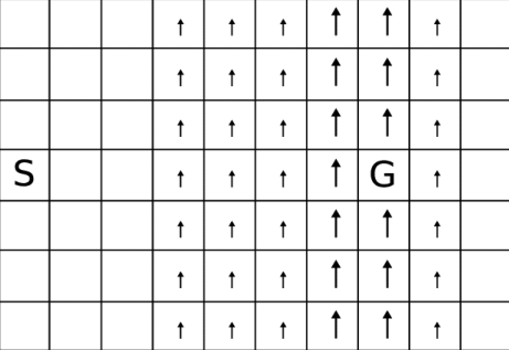
The goal of this project was to study a range of basic principles in tabular, value-based reinforcement learning. The first part focused on Dynamic Programming, which is a bridging method between planning and reinforcement learning. In Dynamic Programming, we have full access to a model of the environment, and we can get the transition probabilities and rewards for any state and action. This guarantees that we will find the optimal solution, given enough iterations.

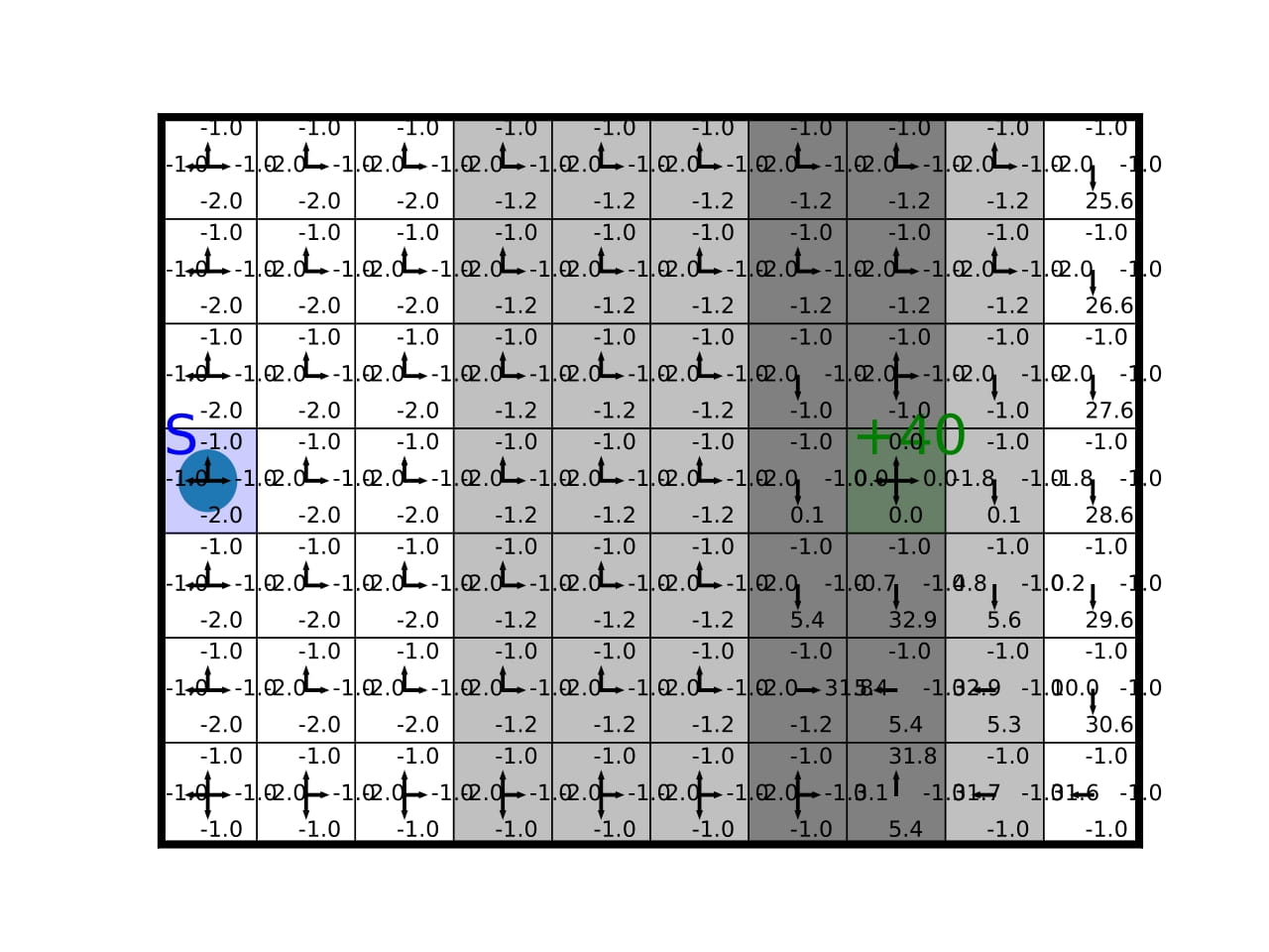
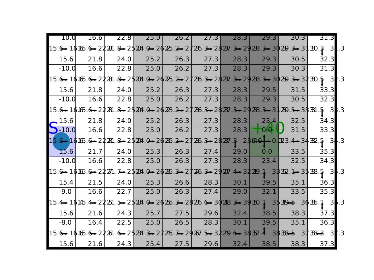
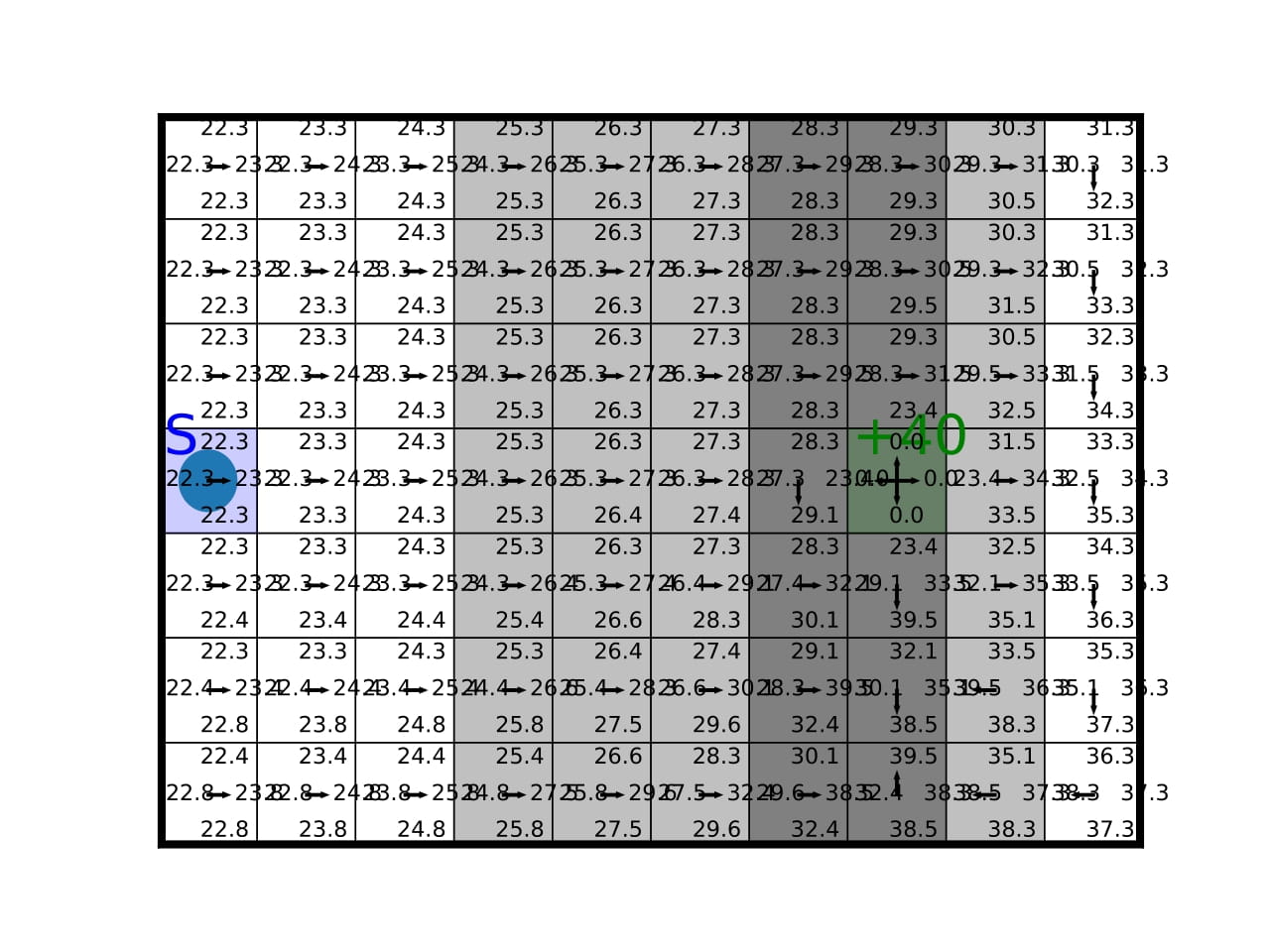
We implemented the Dynamic Programming algorithm and applied it to the Stochastic Windy Gridworld environment. The figure below shows different iterations of the algorithm. The Q-values converge to the optimal policy, after 18 iterations. In the beginning, we see that the values are low in all states, as the agent has not yet learned the optimal policy. After 10 iterations, the agent has learned to navigate the environment and the Q-values are higher and more stable. After 18 iterations, the agent has learned the optimal policy and the Q-values guide the agent to the goal state, in the fewest number of steps, which is 23.3 steps on average. The fact that this number is not an integer is due to the stochastic nature of the environment.

The second part of the project focused on Model-free Reinforcement Learning. We implemented two agents:

• Q-learning
• SARSA The difference between these two agents is that Q-learning is an off-policy algorithm, while SARSA is an on-policy algorithm.

For the exploration strategy, we implemented two methods:

• ε-greedy policy
• softmax (Boltzmann) policy This will help us explore the trade-off between exploration and exploitation by comparing the two methods and the hyperparameters that control the exploration in each method (ε for ε-greedy and temperature for softmax).

Finally we also implemented the n-step back-ups and Monte Carlo back-ups for the Q-learning agent. The n-step back-ups are a generalization of the 1-step back-ups (used by the default Q-learning agent), where we sum more rewards in a trace. The Monte Carlo back-ups are a special case of n-step back-ups, where we sum all rewards until the end of the episode (no bootstrapping).

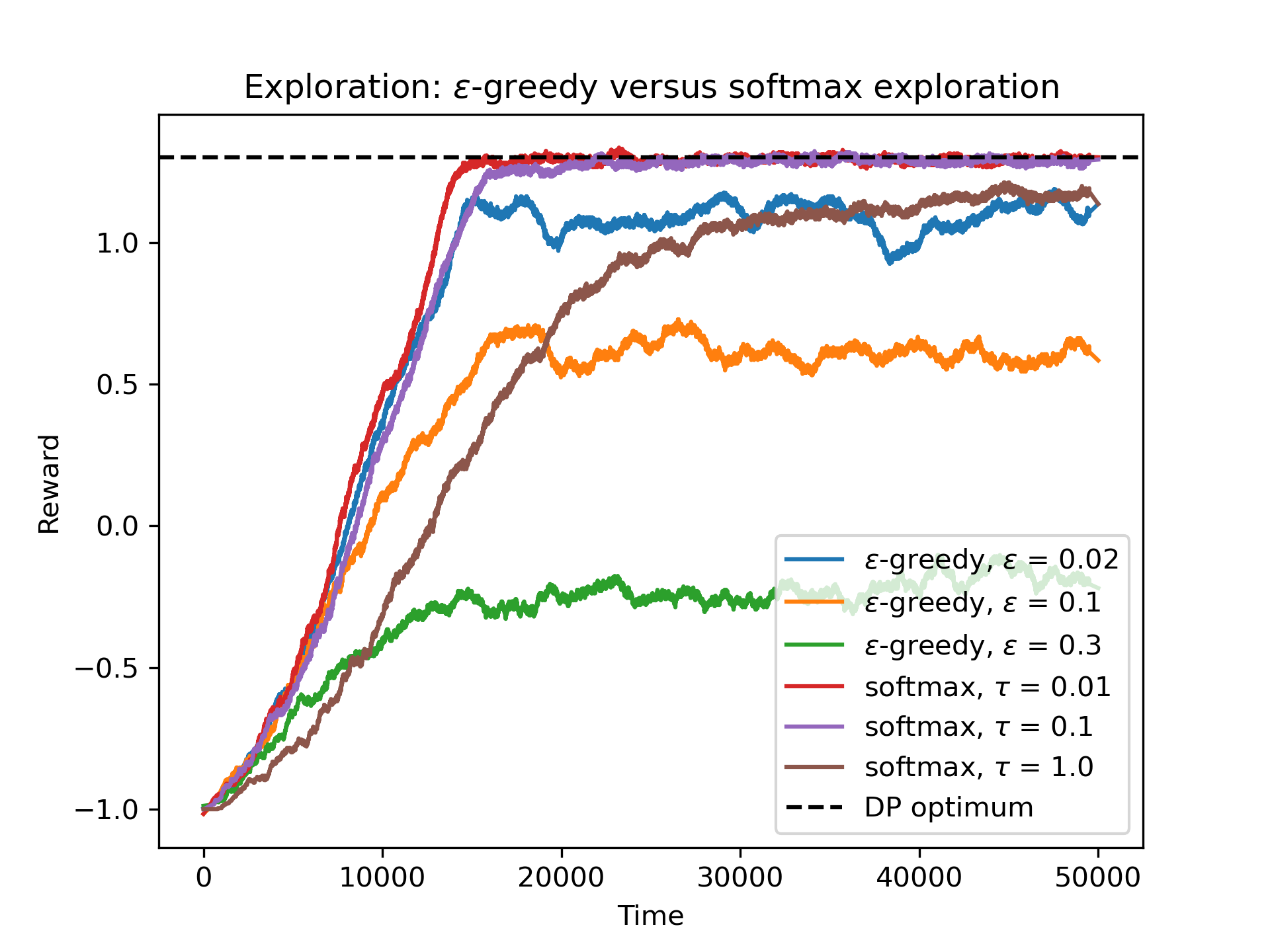
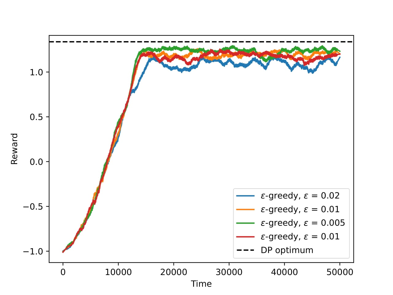
For the first experiment, we compared the exploration strategies. The figure below shows the results of the experiment. On the left we have three different values of ε for the ε-greedy policy and three different values of the temperature for the softmax policy. We can see that the best performance comes from the two lowest values of the temperature (as good as the Dynamic Programming optimum). For this reason on the figure on the right we experimented with even lower values of ε which now perform almost as good as the softmax policy.

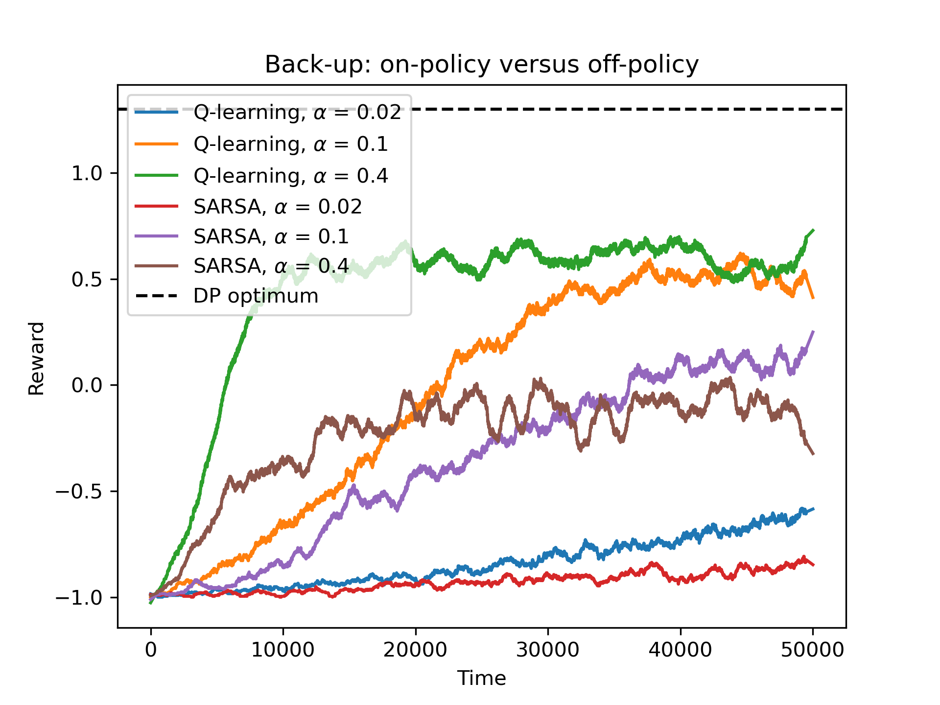
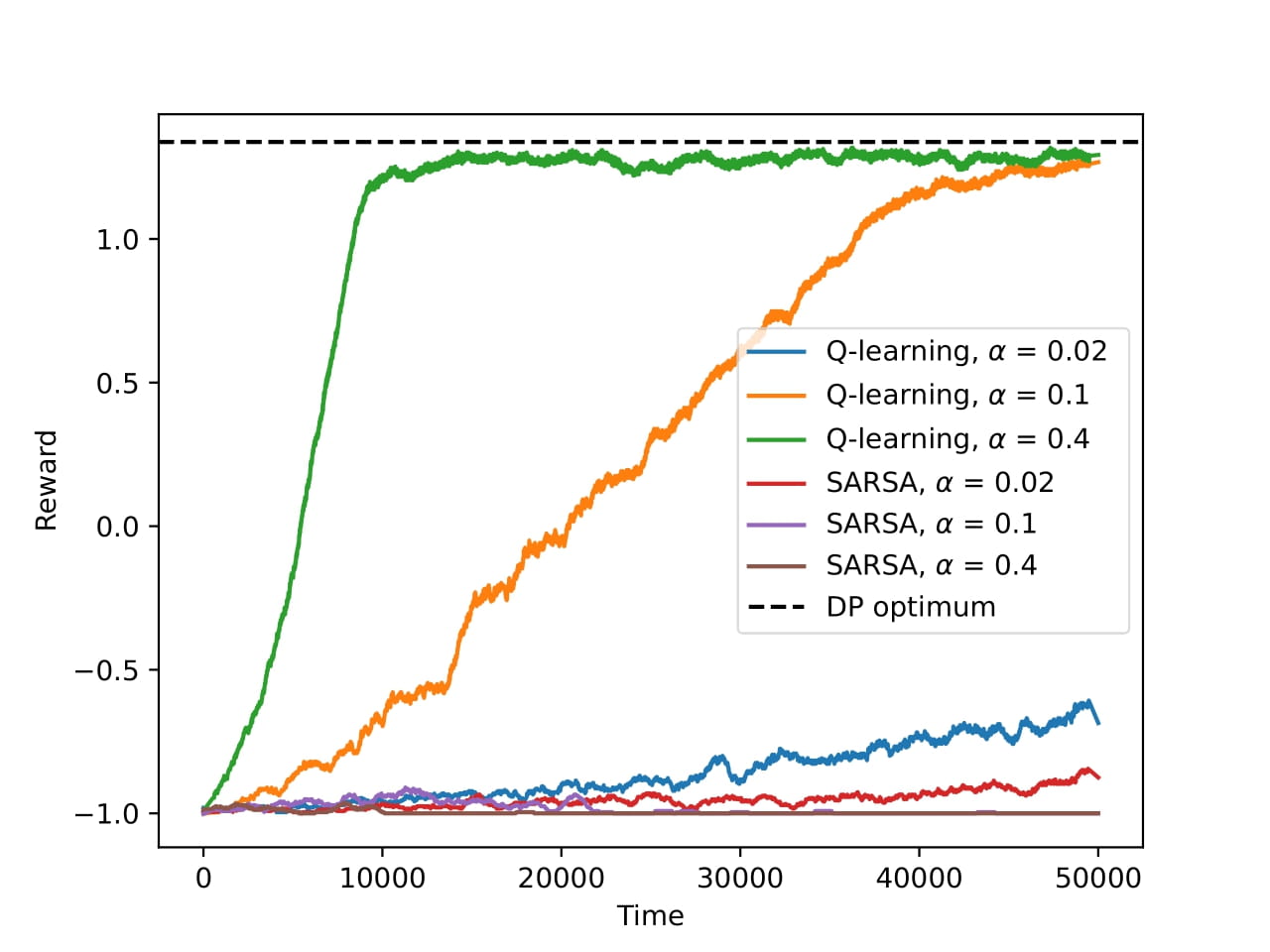
For the second experiment, we compared the on-policy (SARSA) and off-policy (Q-learning) algorithms. The figure below shows the results of the experiment. We can see that the Q-learning algorithm performs better than the SARSA algorithm. The off-policy algorithm, means that the agent learns the optimal policy, even if it is not the one that it is following. The on-policy algorithm, means that the agent learns the policy that the agent is following. For this environment, the off-policy training seems to be more effective.

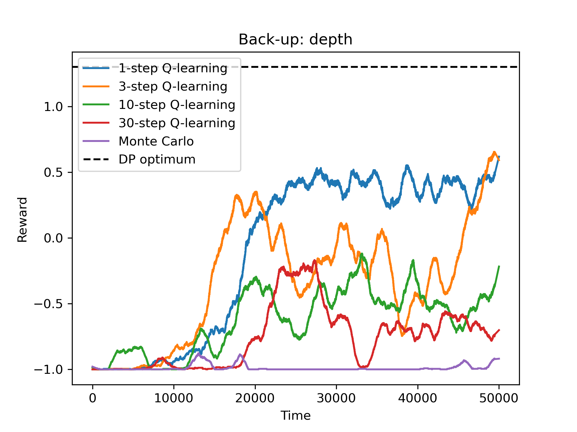
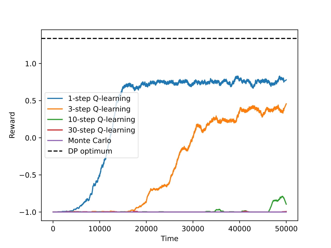
The final experiment compared the n-step back-ups and Monte Carlo back-ups for the Q-learning agent. Keep in mind that the 1-step back-ups are identical to the default Q-learning agent. We see the results of the experiment in the figure below. From the results, we can say that the default Q-learning agent (1-step back-ups) performs better than the n-step back-ups and Monte Carlo back-ups. The smaller the n, the better the performance. This is a classic trade-off between bias and variance. The higher the n, the lower the variance, but the higher the bias. For this particular environment, the lower bias of the 1-step back-ups seems to be more beneficial, despite the higher variance.

Finally, we created some cool animations of the agent’s behavior in the Stochastic Windy Gridworld environment. The three videos show the agent’s behavior at the beginning of training (episodes 3), in the middle of training (episodes 56 and 57), and at the end of training (episodes 179, 180, and 181). The agent uses the Q-learning algorithm with a softmax (Boltzmann) policy with a temperature of 0.01. At the beginning of training, the agent has not yet learned how to navigate the environment and is moving randomly, constantly exploring the world. We have sped up the video 2x because of the many steps the agent takes, to reach the goal state just once. In the middle of training, the agent has greatly improved its performance and is moving more efficiently towards the goal state. It manages to reach the goal state twice within the video. At the end of training, the agent has learned the optimal policy and is moving directly towards the goal state, reaching it in the fewest number of steps. The video is shorter than the other two and yet the agent reaches the goal state three times.

The assignment was a great introduction to reinforcement learning and the different algorithms used in the field. We solved the Stochastic Windy Gridworld environment using Dynamic Programming, Q-learning, and SARSA. We also explored various hyperparameters and strategies for exploration, on-policy vs. off-policy algorithms, and different back-ups. The animations of the agent’s behavior in the environment were a great way to visualize the agent’s learning process and how it improved over time. The full report can be found here. The code for the project is not publicly available, as it is part of the course material. If requested, I can provide parts of the code privately.

Cartpole – Deep Q-Learning

For the second project, we implemented a Deep Q-Learning agent to solve the Cartpole environment from OpenAI Gym using PyTorch. The Cartpole environment is a classic control problem from the reinforcement learning literature (Barto et al., 1983). The environment consists of a cart that can move left or right, and a pole that is attached to the cart. The goal is to balance the pole by applying forces to the cart. The agent receives a reward of +1 for every step taken, including the termination step. The episode ends if the pole angle is greater than ±12°, the cart position is greater than ±2.4 (agent reaches the edge of the display), or the episode length is greater than 500 (maximum number of steps). The action space is discrete with two actions: push the cart to the left or push the cart to the right. The observation space consists of four values: cart position, cart velocity, pole angle, and pole angular velocity.

We implemented the Deep Q-Learning (DQN) algorithm with experience replay and target networks. The DQN agent uses a neural network to approximate the Q-values for each state-action pair. The pseudo-code for the DQN algorithm we implemented is from the book (Plaat, 2022). We implemented DQN using PyTorch. We also implemented a Target Network (TN) to stabilize the learning process and an Experience Replay (ER) buffer to store and sample experiences for training. These features can be turned on or off by the user. We also implemented Double DQN (DDQN) to see if it improves the performance of the agent.

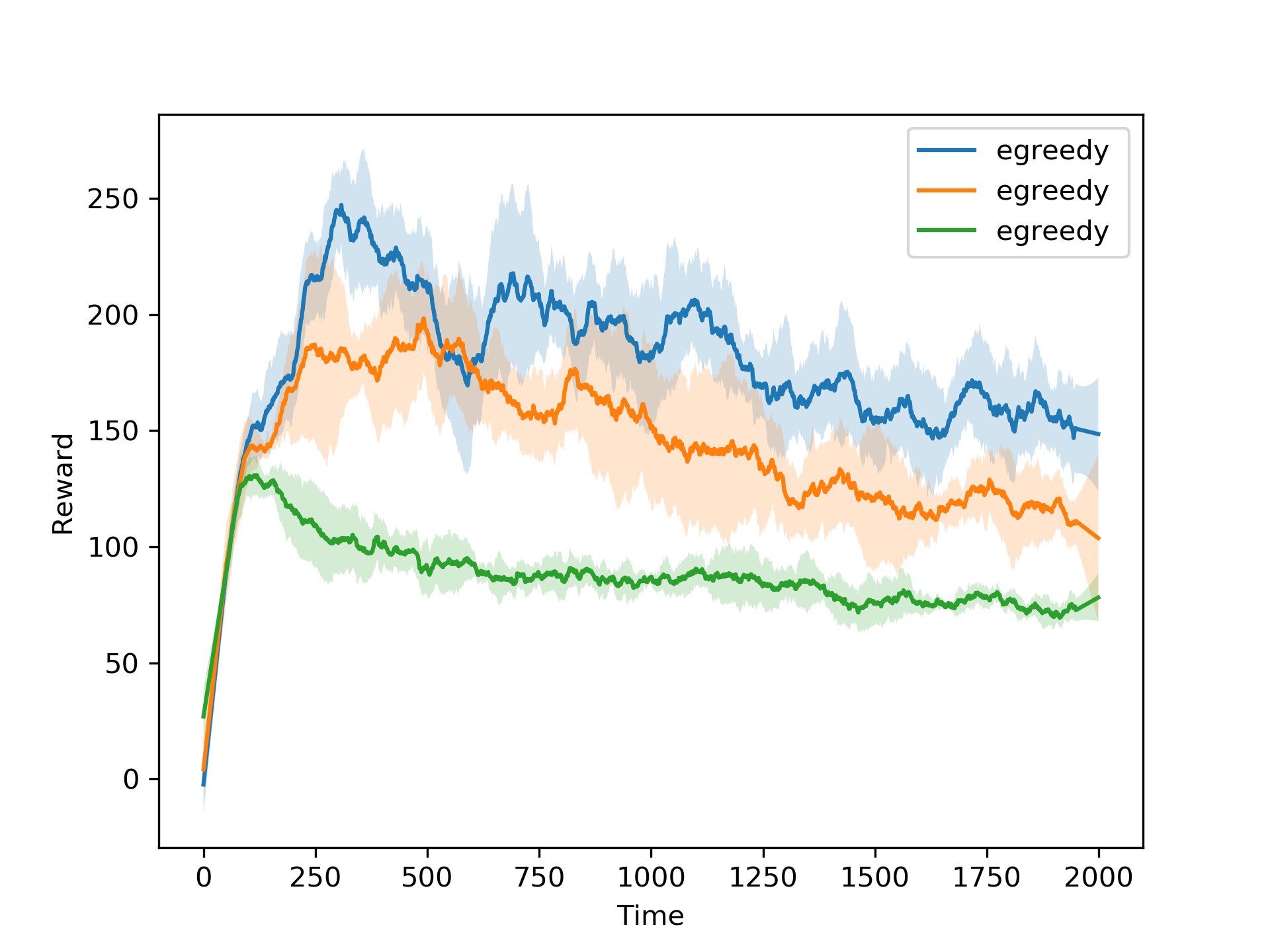
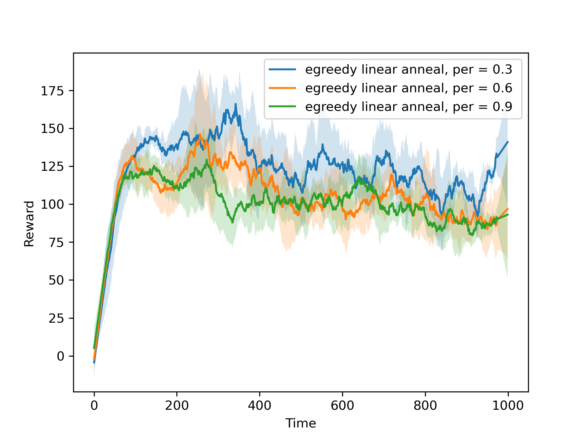
We first use the DQN with both the TN and ER turned on to experiment with different exploration strategies. We compare the ε-greedy and Boltzmann exploration strategies, with different values of ε and temperature. We also experiment with linear annealing of ε and temperature. The results of the experiments are shown in the figures below.

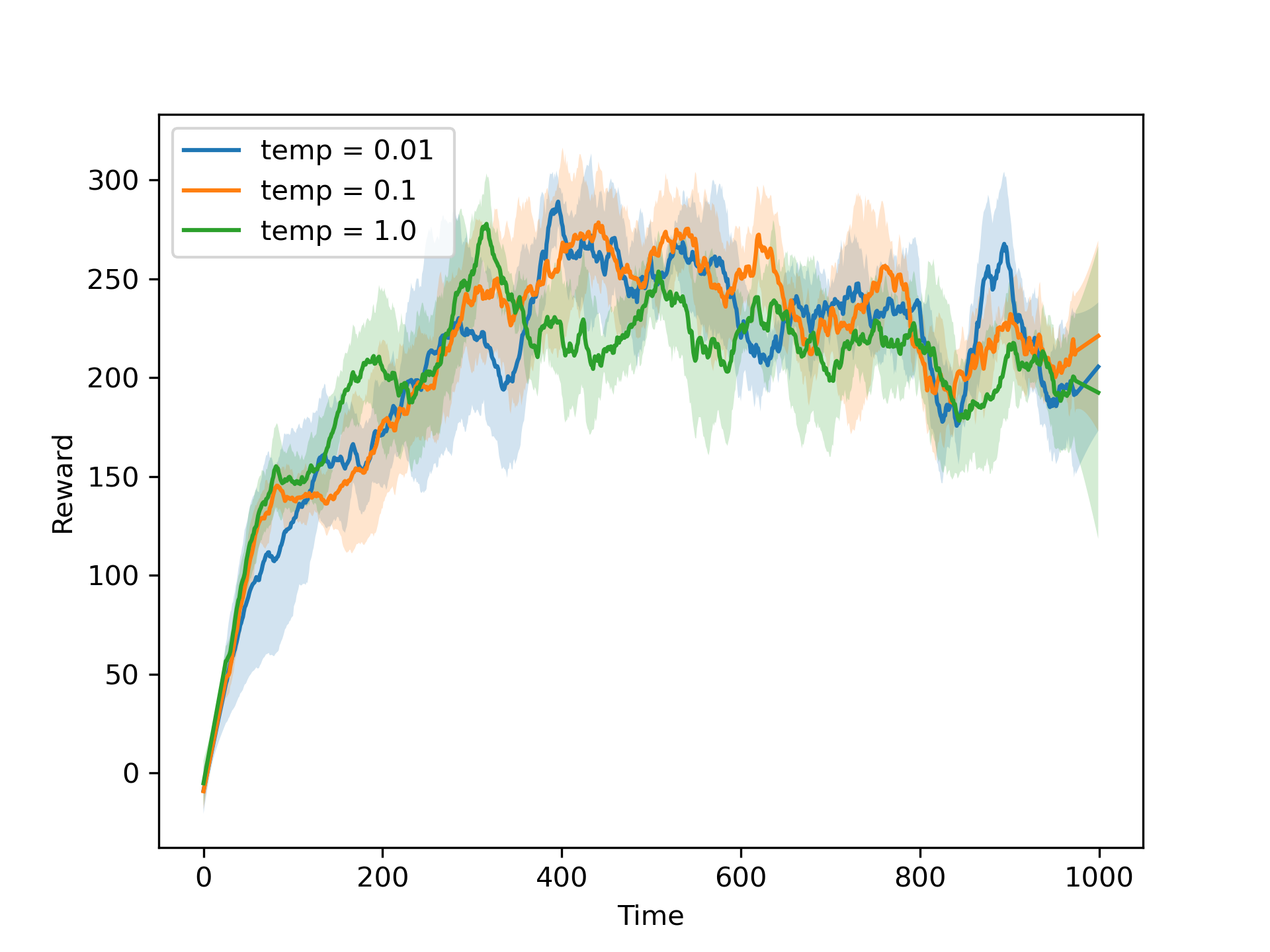
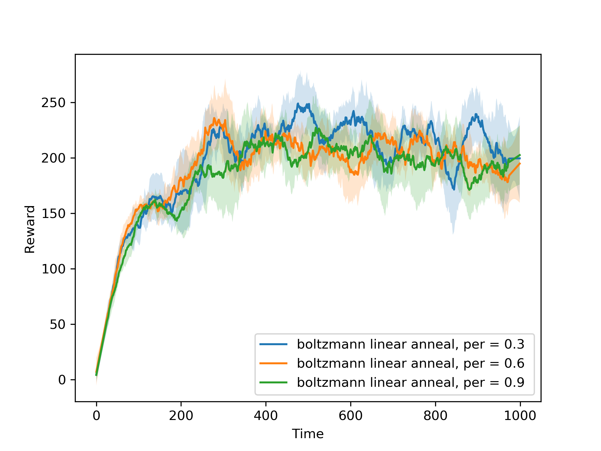
We also implemented a novelty-based exploration strategy, where the agent explores the environment based on the novelty of the state-action pairs. The original code for the novelty-based exploration strategy comes from (Tang et al., 2016), and uses a hash function to calculate the novelty of the state-action pairs. We compare the best performing ε-greedy and Boltzmann strategies with and without linear annealing and the novelty-based exploration strategy. We also compare the performance of the DQN agent with the performance of the DDQN agent. The results of the experiments are shown in the figures below.

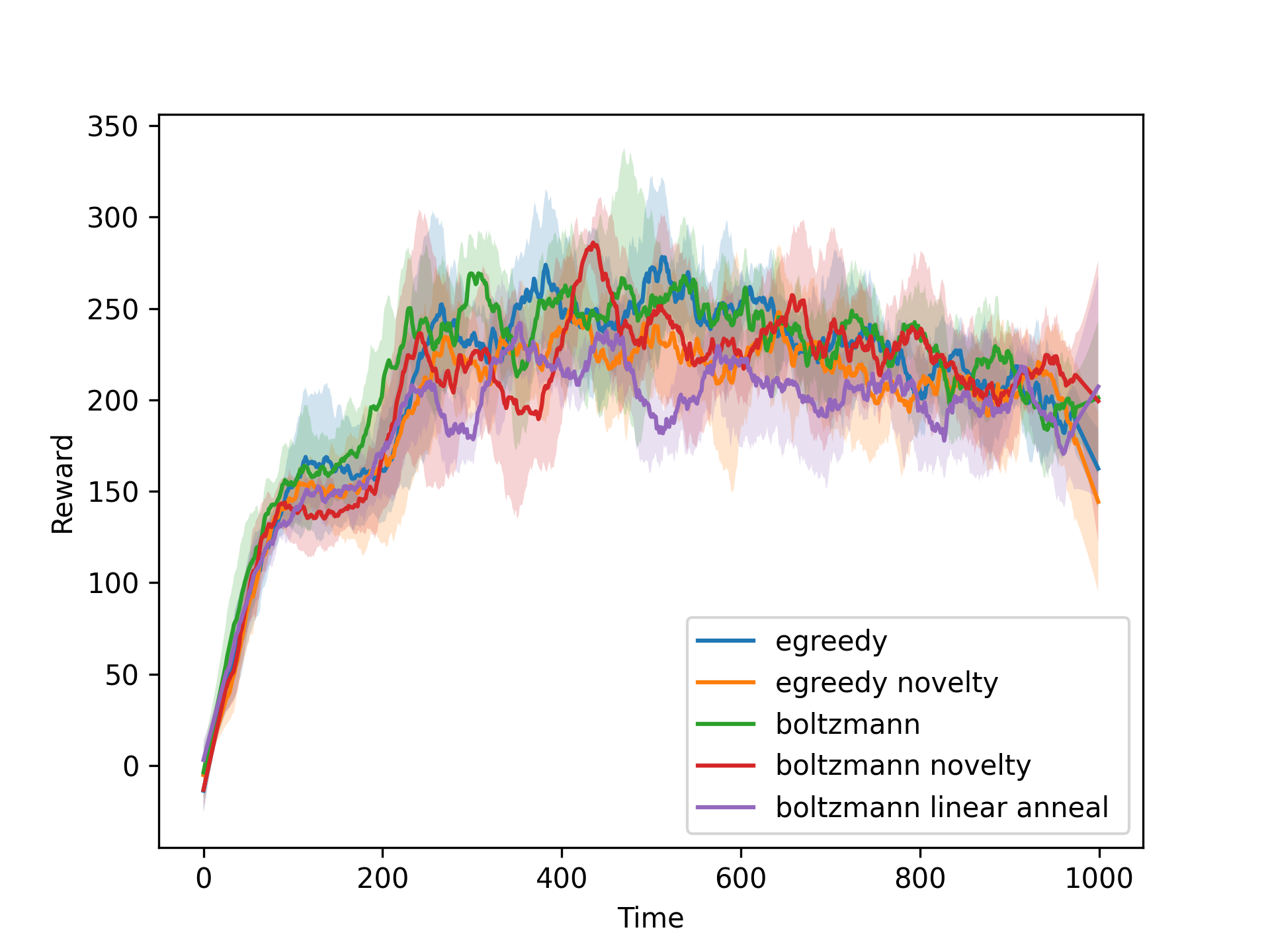
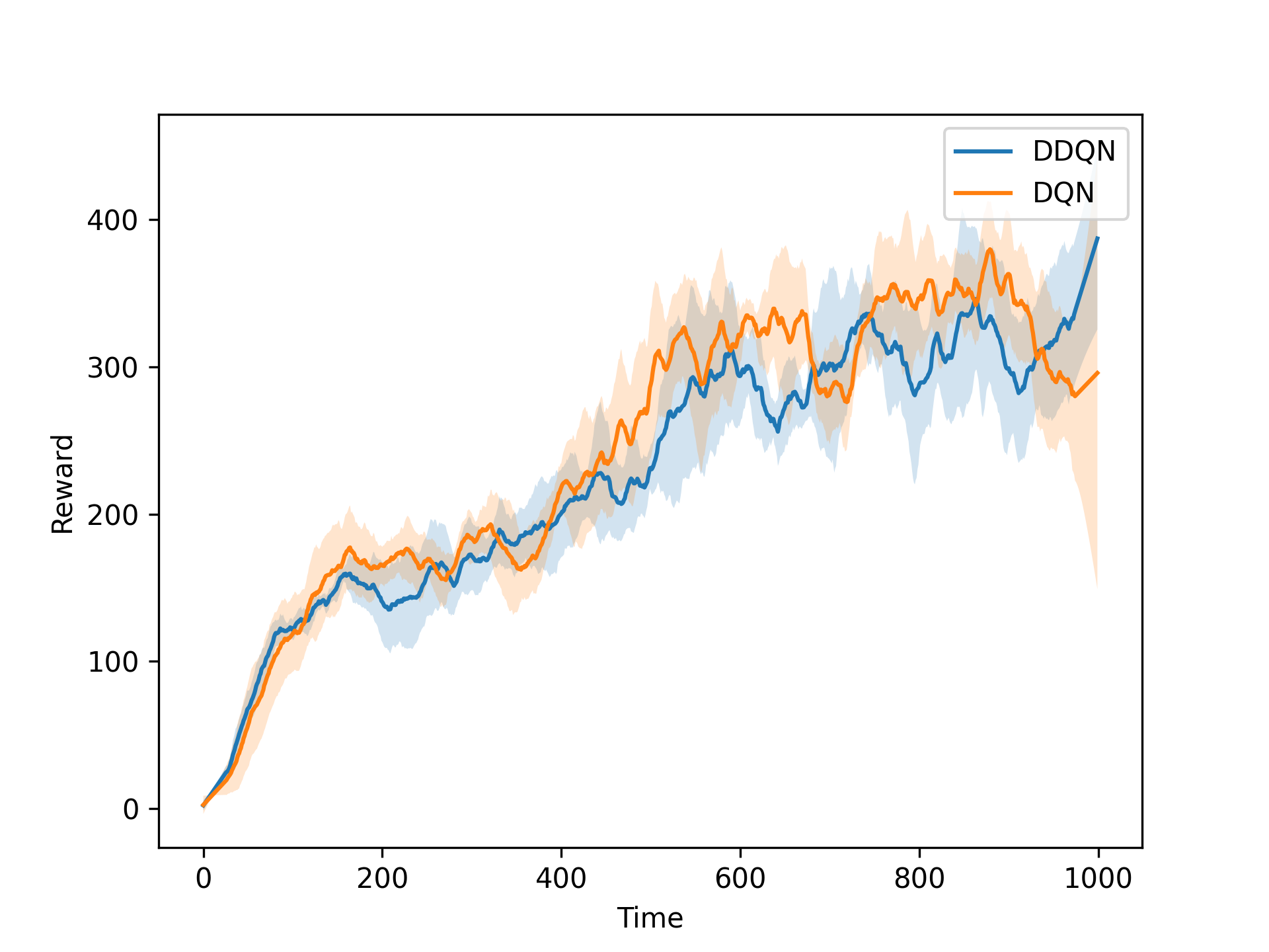
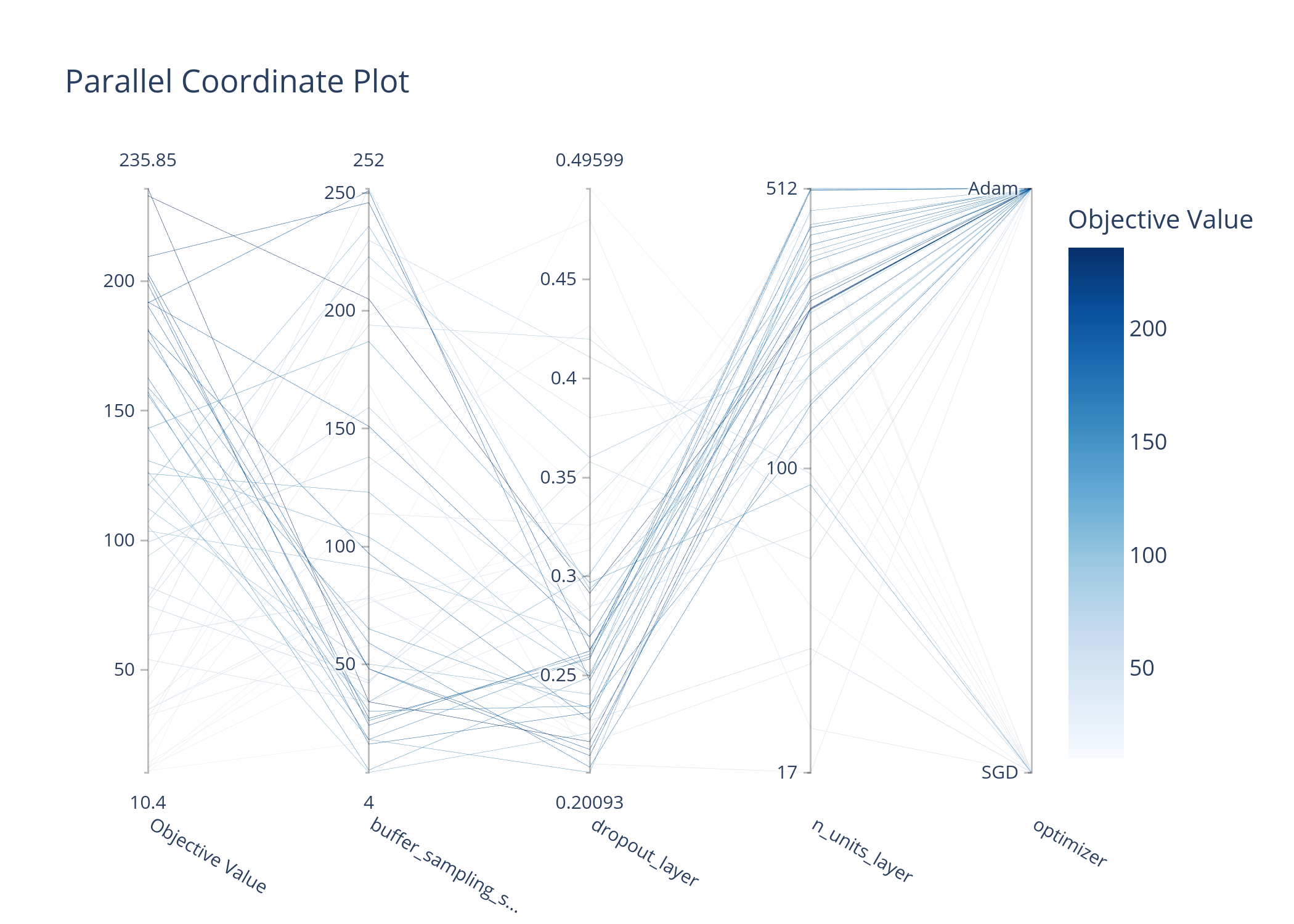
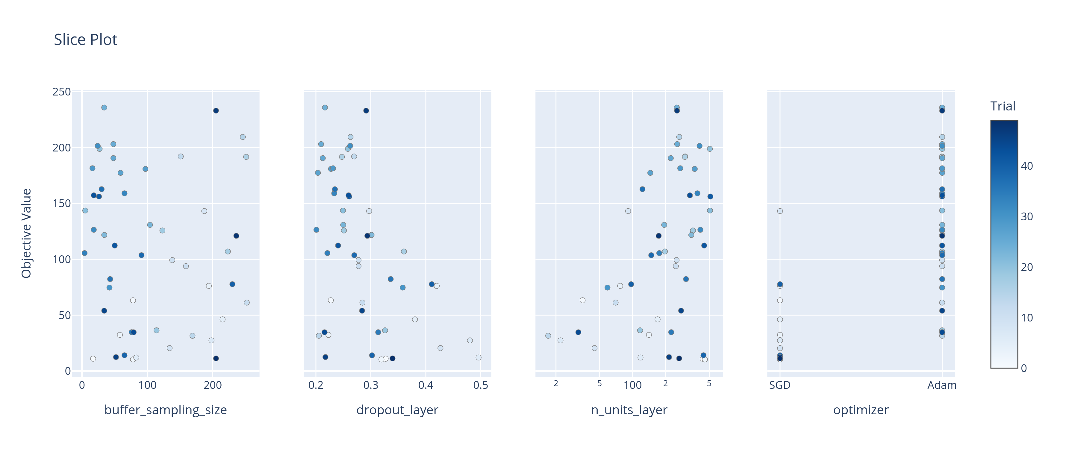
After that we tune the hyperparameters of the DQN agent to find the best performing agent. For the optimazation we use the Optuna library. We can see some figures for the tuning of the most important hyperparameters below.

The best exploration method was the Boltzmann exploration strategy without linear annealing for a temperature of 0.1. We used this value to perform the ablation study where we turned off either or both the TN and ER. The results of the ablation study are shown in the figure below. Note that in the legendd we denote the absence of the TN with “DQN-TN” and the absence of the ER with “DQN-ER”.

We see that although the TN might help with the stability of the learning process, the ER is crucial for the performance of the agent. The best performing agent was the DQN agent with both the TN and ER turned on.

Finally, we train the best performing agent and save the weights of the neural network at various stages of training. We then evaluate the agent using the saved weights and create some cool video animations of the agent’s behavior in the Cartpole environment. The videos show the agent’s behavior at the beginning of training (episodes 20), in the middle of training (episodes 200 and 400), and at the end of training (episodes 800). We see how the agent goes from completely poor performance at the beginning of training to a perfect performance at the end of training. At mid-training, the agent seems to struggle more staying within the limits of the environment, and seems to be doing better at balancing the pole. The videos are shown below.

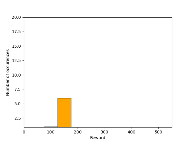
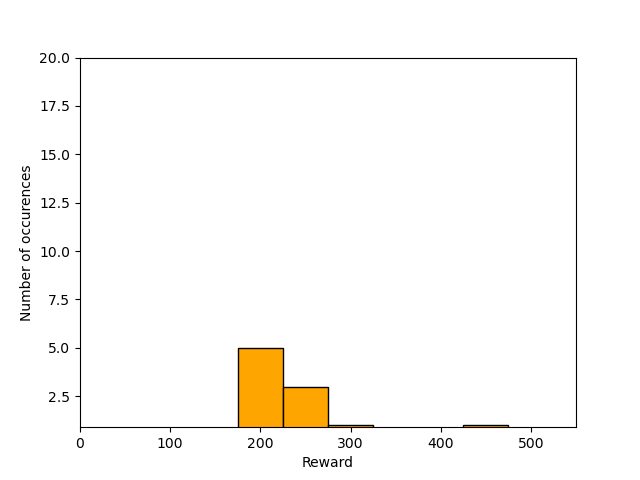
We can also create histograms of the rewards obtained by the agent during evaluation after 200, 400, and 800 episodes of training. The histograms are shown below. We can see that at the end of training, the agent is consistently obtaining the maximum reward of 500, which means that the agent is balancing the pole for the maximum number of steps (500 steps).

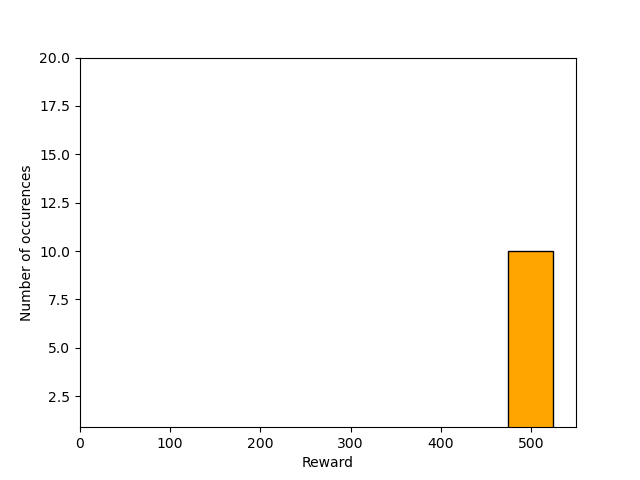
Overall, we were successful in training a Deep Q-Learning agent to solve the Cartpole environment. We experimented with different exploration strategies, hyperparameters, and ablated the TN and ER. We found that the best performing agent was the DQN agent with both the TN and ER turned on, using the Boltzmann exploration strategy with a temperature of 0.1. We also implemented the DDQN agent and compared its performance with the DQN agent. We found that the DDQN agent performed at the same level as the DQN agent. The full report can be found here. The code for the project is not publicly available, as it is part of the course material. If requested, I can provide parts of the code privately.

Catch – Actor-Critic

In this assignment we worked with a new environment called Catch, which is an extension from the Catch environment in (Osband et al., 2019). The environment consists of a paddle that moves left or right to catch balls that drop from the top of the screen. It has a 7x7 grid, and the agent can move the paddle left, right, or stay idle. The agent receives a reward of +1 when catching a ball, a reward of -1 when missing a ball, and a reward of 0 otherwise. The episode ends when the agent reaches the maximum number of steps (default is 250 steps) or misses the maximum number of balls(default is 10 balls). The observation space can be either a vector with the xy-locations of the paddle and the lowest ball, or a binary two-channel pixel array with the paddle location in the first channel and all balls in the second channel. The speed of dropping new balls can be adjusted, as well as the size of the grid.

We implemented three agents in this project:

• REINFORCE
• Actor-Critic
• Proximal Policy Optimization (PPO)

All these agents use a policy-based algorithm, which is a different approach from the value-based algorithms (DQN and DDQN) used in the previous projects. The policy-based algorithms directly learn the policy, which is a mapping from states to actions, without learning the value function. The REINFORCE agent uses the Monte Carlo policy gradient method to update the policy. The Actor-Critic agent uses an actor network to learn the policy and a critic network to learn the value function. The PPO agent uses the Proximal Policy Optimization algorithm to update the policy, which utilizes a clipped objective function to prevent large policy updates.

For the Actor-Critic agent, we also implemented a Baseline and Bootstrapping. The hyperparameters, we experimented with many different values to find the best performing agent. We performed an ablation study to compare the performance of the Actor-Critic agent with and without the Baseline and Bootstrapping, as well as the REINFORCE agent. The results of the ablation study are shown in the figure below.

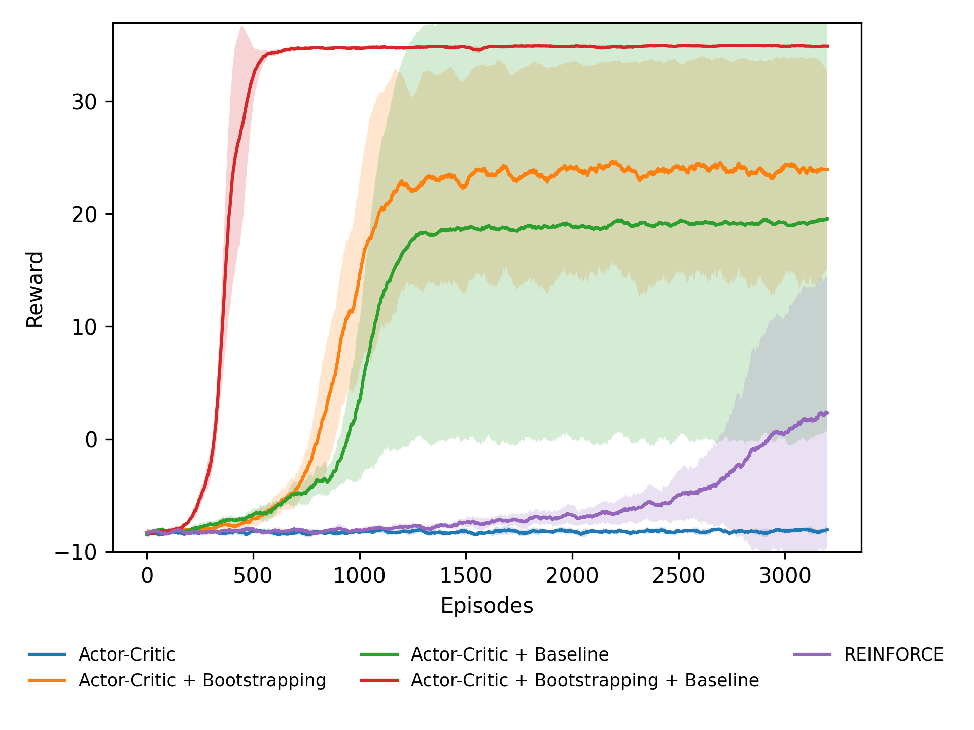
As we can see from the results, the Actor-Critic agent greatly improves by using the Baseline and Bootstrapping. The vanilla Actor-Critic agent (no Baseline and Bootstrapping) is not able to learn at the environment. The REINFORCE agent performs better than the vanilla Actor-Critic agent, but not as good as the Actor-Critic agent with either the Baseline or Bootstrapping. The best performing agent is the Actor-Critic agent with both the Baseline and Bootstrapping turned on.

Next we experiment with the vector and pixel (default) input for the Catch environment. We also compare the PPO agent for different values of the ε-clip parameter with the Actor-Critic agent. We experiment with different grid sizes and speeds for the Actor-Critic agent. We also use the Actor-Critic agent to solve the Cartpole environment (see the previous project). All these experiments are shown in the figures below.

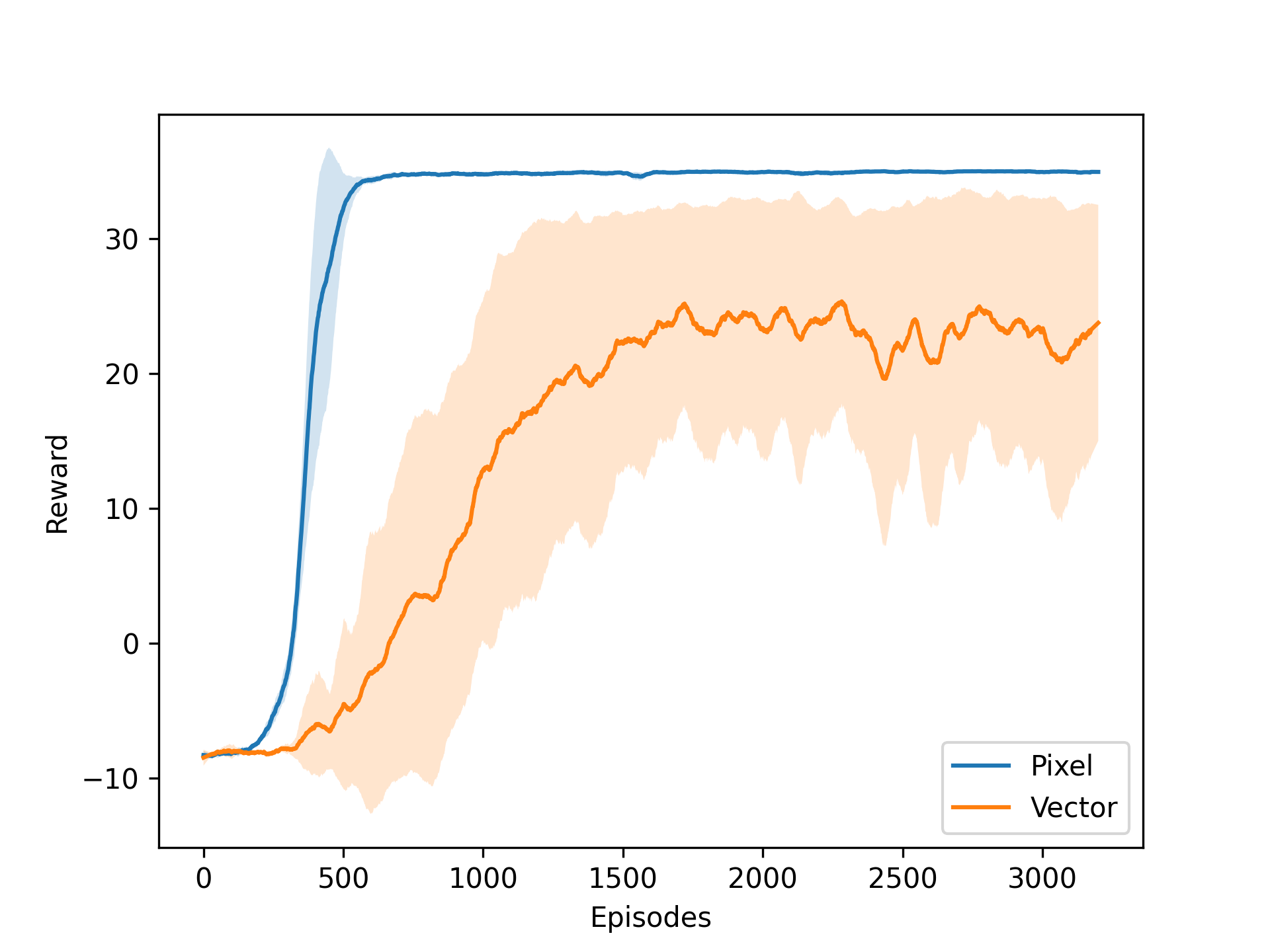
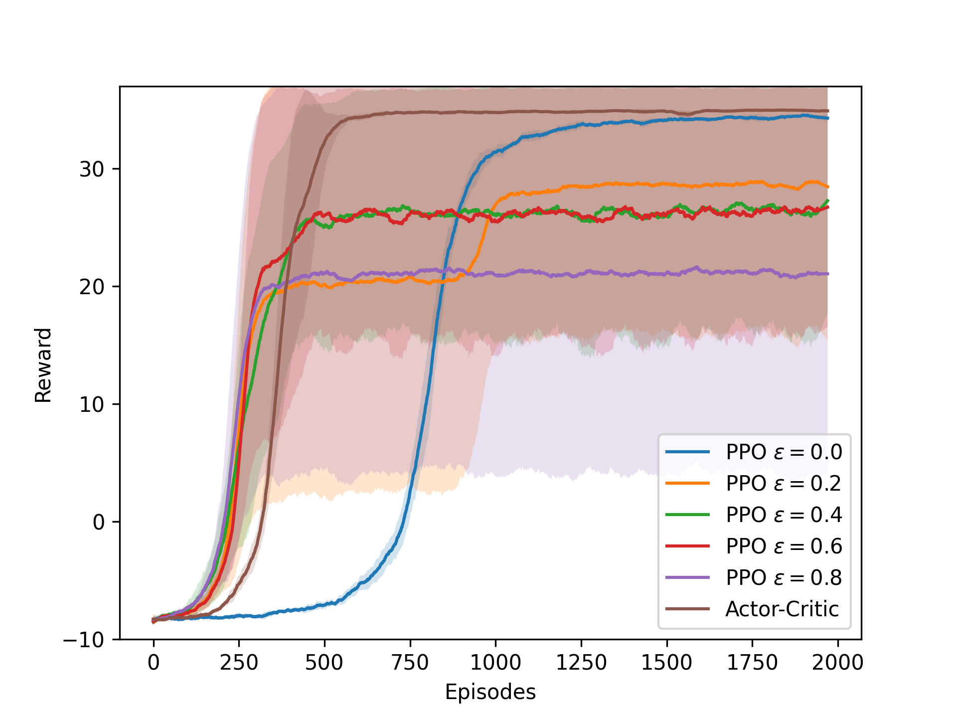
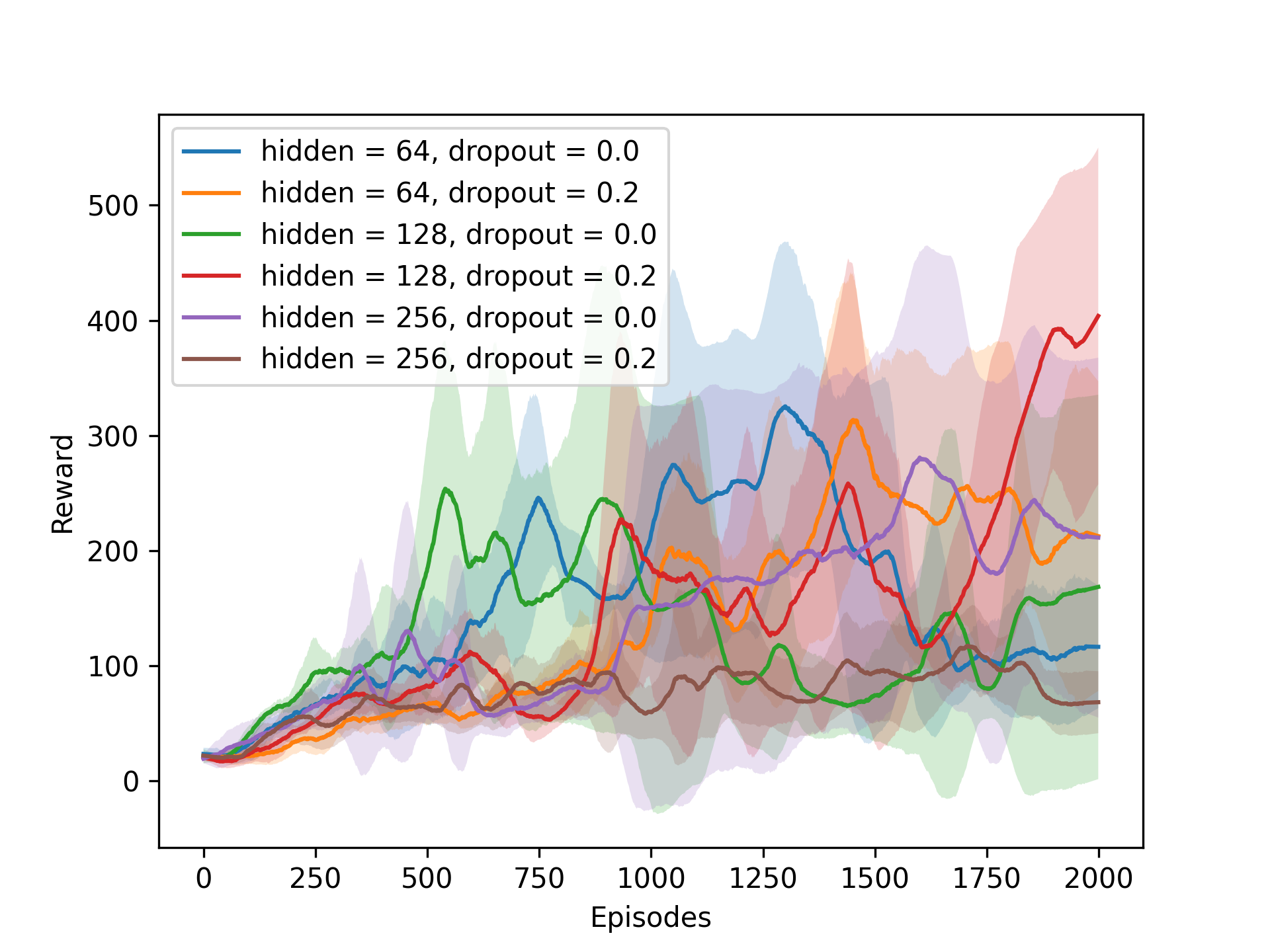
As we can see the vector input makes the learning process more unstable, and does not reach the performance of the default pixel input. The PPO agent performs better with a lower value of the ε-clip parameter, but is slower to learn than the Actor-Critic agent. For the Cartpole environment, the Actor-Critic agent shows some learning progress, but is not able to solve the environment. It should be noted that we did not spend much time tuning the hyperparameters for the Cartpole environment, as the focus was on the Catch environment, so the results are still promising.

After that we experimented with some environment variations. We used the best performing Actor-Critic agent to solve the environment with different grid sizes, speeds, and combinations of grid sizes and speeds. When the ball speed is greater than 1.0 (default), the new ball drops before the previous ball reaches the bottom row. The opposite is true when the ball speed is less than 1.0. The results of the experiments are shown in the figures below. To compare the performance of the agent, we used the fraction of caught balls for each episode.

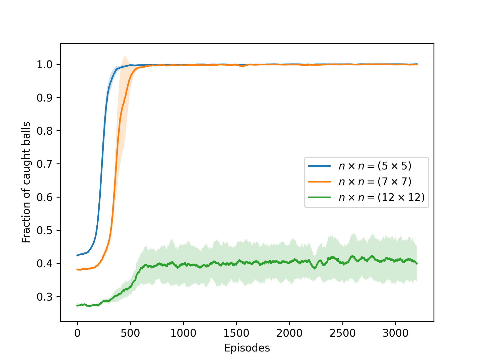
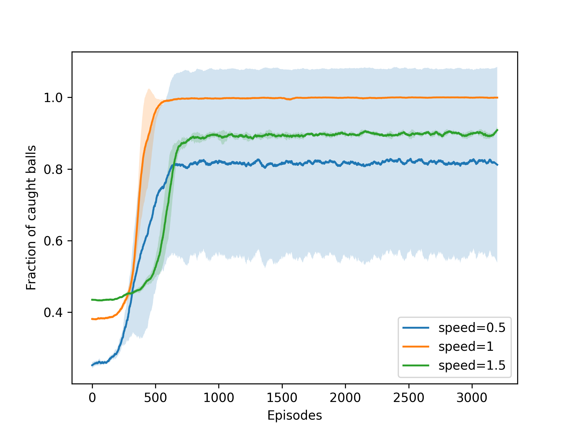
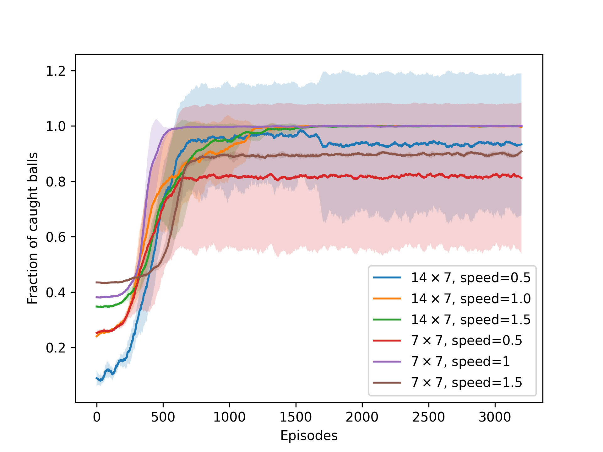
As we can see, making the grid smaller helped the agent to learn faster, but increasing it too much made the learning process unstable and suboptimal. Increasing the speed of the balls also lowered the performance of the agent, it was however expected, since it was no longer possible to catch all the balls, even when playing perfectly. What is surprising is that a slower speed for the balls made the learning process very unstable, with some runs reaching the optimal performance, and others being very far from it.

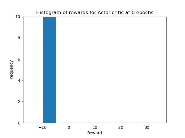
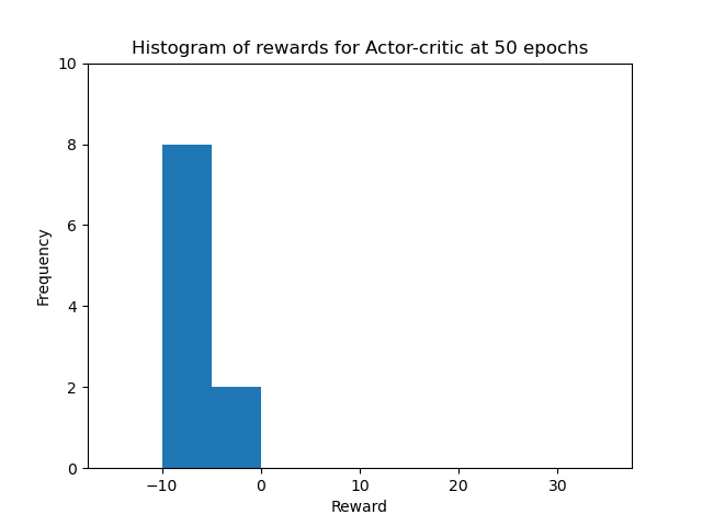
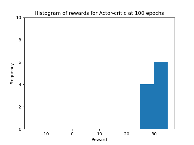
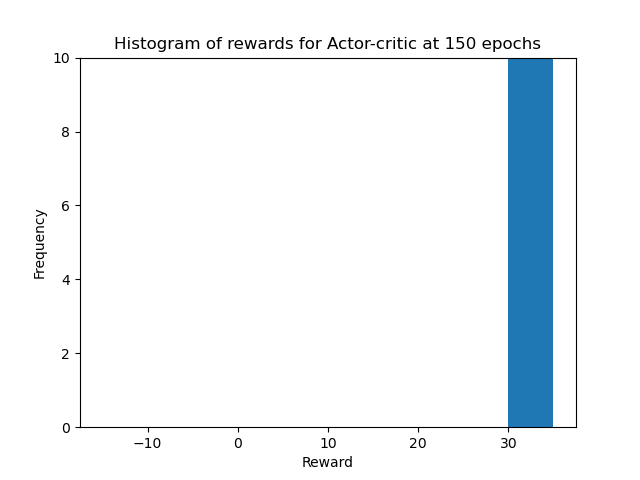
Finally, we created some nice video animations of the performance of our best agent (Actor-Critic with Baseline and Bootstrapping) at various stages of the learning process. The videos show the agent’s behavior at the start of training (after 0 epochs), in the first stages of training (after 50 epochs), in the middle of training (after 100 epochs), and at the end of training (after 150 epochs). The agent kept learning after that, but the performance did not improve as it had already reached the optimal performance. For each evaluation we turned off the exploration and training, and the agent played 10 episodes. The videos only show 5 episodes for the first two stages and 3 episodes for the last two stages, to keep the videos short. The videos are shown below.

We can see that at 0 epochs of training, the agent is moving randomly and is only able to catch a few balls, just by chance. After 50 epochs of training, the agent still moves more or less randomly, but is able to catch some more balls. After 100 epochs of training, the agent has learned to move more efficiently and is able to catch most of the balls. At 150 epochs of training, the agent has learned the optimal policy and is able to catch all the balls. We can also see that in the histograms of the rewards obtained by the agent during evaluation in all four stages of training for the 10 episodes. The histograms are shown below.

In conclusion, we were able to train an Actor-Critic agent to solve the Catch environment. We experimented with different hyperparameters, ablated the Baseline and Bootstrapping, and compared the performance of the Actor-Critic agent with the REINFORCE agent. We also experimented with the vector and pixel input for the Catch environment, and compared the PPO agent with the Actor-Critic agent. We experimented with different grid sizes and speeds for the Catch environment, and used the Actor-Critic agent to try to solve the Cartpole environment. The full report can be found here. The code for the project is not publicly available, as it is part of the course material. If requested, I can provide parts of the code privately.

References

2022

1. Deep Reinforcement Learning, a textbook

   Aske Plaat

   arXiv e-prints, Jan 2022

2019

1. Behaviour Suite for Reinforcement Learning

   Ian Osband, Yotam Doron, Matteo Hessel, John Aslanides, and 10 more authors

   arXiv e-prints, Aug 2019

2018

1. Reinforcement Learning: An Introduction

   Richard S. Sutton, and Andrew G. Barto

   Aug 2018

2016

1. #Exploration: A Study of Count-Based Exploration for Deep Reinforcement Learning

   Haoran Tang, Rein Houthooft, Davis Foote, Adam Stooke, and 5 more authors

   arXiv e-prints, Nov 2016

1983

1. Neuronlike adaptive elements that can solve difficult learning control problems

   Andrew G. Barto, Richard S. Sutton, and Charles W. Anderson

   IEEE Transactions on Systems, Man, and Cybernetics, Nov 1983